
数据挖掘论文范文
Statistical prediction of EI Nino and Hurricanes来源:人大经济论坛论文库 作者:Kaiqing Fan 时间:2016-05-25
Statistical prediction of EI Nino and Hurricanes
Kaiqing Fan
Introduction
We have the data set with the numbers of Atlantic Basin tropical storms and hurricanes for each year from 1950 to 1997. The data set include year, EI Nino temperature, West Africa, Storms, Hurricanes Storm index. Storm index is an index of overall intensity of the hurricanes season. We take on the values -1, 0, and 1 according to whether the EI Nino temperature is cold, warm and neutral; and a variable including whether West Africa was wet or dry that year. It is thought that the warm phase of EI Nino suppresses hurricanes and while a cold phase encourages them. It is also thought that wet year in West Africa often bring more hurricanes.
Our Purpose is to analyze the data to describe the effect of EI Nino on 1) the number of tropical storms, 2) the number of hurricanes, and 3) the storm index after accounting for the effects of West Africa wetness and for any time trends, if appropriate.
In this report I take the number of tropical storms as y1 , and the number of hurricanes as y2 , the storm index as y3 , and the effects of West Africa wetness as x1 , and the effect of EI Nino as x2.
And because the variable storm index is an index of overall intensity of the hurricane season, I take the storm index as Y, West Africa wetness as x1, the temperature of EI Nino as x2, hurricanes as x3, tropical storm as x4, do another multiple regression.
Also we have the data set as following:
Year Storms Hurricanes NTC El Nino West Africa
1950 13 11 243 Cold Wet
1951 10 8 121 Warm
1952 7 6 97 Wet
1953 14 6 121 Warm Wet
...
1994 7 3 37 Warm
1995 19 11 237 Cold Wet
1996 13 9 198 Cold
1997 7 3 54 Warm Dry
Non-technical Analysis
1, The effect of EI Nino (x2) on the number of tropical storms (y1) after accounting for the West Africa wetness (x1).
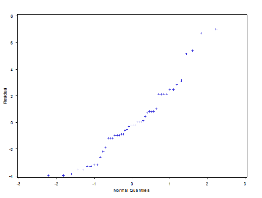
Let us check the data set. It is clear that the plot of residuals vs predicted values is half of megaphone pattern, it may suggest non-constant variance. And also there may have two outliers in this plot. In the normal probability plot of residuals, there is right long tail it means that this plot is not normal distribution.
SAS output gives us the multiple regression is : y1 = 8.86046 + 1.42765x1 – 1.68770x2
So this multiple regression is not very good x1 and x2 can only explain 30.32% of the total y1.
2, The effect of EI Nino (x2) on the number of hurricanes (y2) after accounting for the West Africa wetness (x1).
In this plot of res*pred, there is an extreme value, and the shape is mild curvilinear pattern, it may suggest non-linearity of regression function.
SAS output gives us the multiple regression is : y2 = 5.28698 + 1.23473x1 – 1.22990x2
But this multiple regression is not very good x1 and x2 can only explain 33.01% of the total y2.
3, The effect of EI Nino (x2) on the number of hurricanes (y3) after accounting for the West Africa wetness (x1).
In this plot of res*pred, there may have several outliers, they challenge the correct assumptions of these data set. In the normal probability plot of residuals, it almost looks like a linear pattern, only there is a long tail, which may suggest outliers.
SAS output gives us the multiple regression as : y3 = 83.79053 + 45.61415x1 – 28.95941x2
But this multiple regression is not very good x1 and x2 can only explain 49.51% of the total y3.
4, In the plot of residual*pred, there is megaphone pattern that may suggest non-constant variance.
Then, SAS output gives us the multiple regression is : y = -0.39443 + 25.95350x1 – 9.37555x2 + 15.92308x3
But this multiple regression is not very good x1 , x2 and x3 can explain 81.68% of the total Y.
The interaction of x3 and x1 is not high, the interaction of x3 and x2 is also not high.
5, The plot of res*pred suggests non-constancy variance.
R-square is 72.46%, it means that the x1, x2 and x4 can explain 72.46% of total Y.
The multiple regression model is Y= -2.03282 + 31.78576x1 – 12.61216x2 +9.68610x4,
but it is significant that we can claim that b0=0.
6, the plot of res*pred suggests non-constancy variance.
When we put another variable storms (here takes it as x4) into the Y model,
The multiple regression model is: Y = -8.35152 + 25.63282x1 – 8.41958x2 + 13.41190x3 + 2.39645x4.
But we can drop the x4 in the model. And we also can claim with significance that b1=0, and b4=0.
Conclusions
From analysis shown above, we can get the following results:
1, The data set is not the correct assumptions of multiple regression, so we can not get a good fitted model easily. Using these models: y1 = 8.86046 + 1.42765x1 – 1.68770x2 and y2 =5.28698 + 1.23473x1 – 1.22990x2 and y3 = 83.79053 + 45.61415x1 – 28.95941x2, we can only explain the response variables of y1 and y2 and y3 by 30.32%, 33.01% and 49.51%.
If we want to explain the number of tropical storms and the number of hurricanes and the storm index, we need choose other model or think of other variables that may explain these three variables well.
2, The full multiple regression model is: Y = -8.35152 + 25.63282x1 – 8.41958x2 + 13.41190x3 + 2.39645x4.
When we think of the storm index as response variable Y, it is not very good for us to keep every variable such as west Africa wetness x1 , EI Nino temperature x2, hurricanes x3 and tropical storms x4, because x3 and x4 is correlated by 83.156%, that is , there is 83.156% of information of x3 that is already included in x4.
3, Comparing with multiple regressions between y = -0.39443 + 25.95350x1 – 9.37555x2 + 15.92308x3 and Y= -2.03282 + 31.78576x1 – 12.61216x2 +9.68610x4, we would like to choose the first model, since R-square of the first model is 81.68% compared with the second model R-square of 72.46%.
Technical analysis: Appendix of non-technical anysis
1, the plot of residuals vs predicted values is half of megaphone pattern, it may suggest non-constant variance. And also there may have two outliers in this plot.
Plot of res*pred. Symbol used is 'r'.
‚
‚
‚
8 ˆ
‚
‚ r
‚ r
‚
6 ˆ
‚
‚ r r
‚
‚
R 4 ˆ
e ‚
s ‚ r
i ‚ r
d ‚ r
u 2 ˆ r
a ‚
l ‚ r
‚ r r
‚ r
0 ˆ r r r
‚ r r
‚ r r r
‚ r
‚
-2 ˆ r r
‚
‚ r
‚ r r
‚ r
-4 ˆ r r
‚
Šƒˆƒƒƒƒƒƒƒƒƒƒƒƒˆƒƒƒƒƒƒƒƒƒƒƒƒˆƒƒƒƒƒƒƒƒƒƒƒƒˆƒƒƒƒƒƒƒƒƒƒƒƒˆƒƒƒƒƒƒƒƒƒƒƒƒˆƒƒƒƒƒƒƒƒƒƒƒƒƒ
7 8 9 10 11 12
Predicted Value of y
NOTE: 19 obs hidden.
In the normal probability plot of residuals, use the fat pencil we can get that there is right long tail it means that this plot is not normal distribution.
Pic 1
y1 = 8.86046 + 1.42765x1 – 1.68770x2, the p-value of west Africa x1 is 0.1122, in the t-test of H0: b1=0 vs H1: b1≠0, we keep H0 that b1=0.
Parameter Estimates
Parameter Standard
Variable Label DF Estimate Error t Value Pr > |t|
Intercept Intercept 1 8.86046 0.51621 17.16 <.0001
west_africa west#africa 1 1.42765 0.88129 1.62 0.1122
temperature temperature 1 -1.68770 0.52254 -3.23 0.0023
R-square is 0.3032 , it means x1 and x2 can explain 30.32% of the y1. So the multiple regression function is not very good one, we may need add more variables or try other regression function.
Root MSE 2.74740 R-Square 0.3032
Dependent Mean 9.39583 Adj R-Sq 0.2722
Coeff Var 29.24067
2, In this plot of res*pred, there is an extreme value, and the shape is mild curvilinear pattern, it may suggest non-linearity of regression ffunction.
Plot of res*pred. Symbol used is 'r'.
‚
‚
‚
6 ˆ
‚
‚ r
‚
‚
‚
4 ˆ r
‚ r
‚ r
‚
R ‚ r
e ‚ r
s 2 ˆ r
i ‚ r
d ‚ r
u ‚ r
a ‚ r
l ‚ r r
0 ˆ r
‚ r
‚ r r
‚ r
‚ r
‚ r r
-2 ˆ r
‚ r
‚ r r
‚
‚
‚
-4 ˆ
‚
Šƒˆƒƒƒƒƒƒƒƒƒƒƒƒƒƒƒˆƒƒƒƒƒƒƒƒƒƒƒƒƒƒƒˆƒƒƒƒƒƒƒƒƒƒƒƒƒƒƒˆƒƒƒƒƒƒƒƒƒƒƒƒƒƒƒˆƒƒƒƒƒƒƒƒƒƒƒƒƒƒ
4 5 6 7 8
Predicted Value of y
NOTE: 23 obs hidden.
R-square is 33.01%, it means that x1 and x2 can only explain 33.01% of the total y2.
Root MSE 1.97868 R-Square 0.3301
Dependent Mean 5.75000 Adj R-Sq 0.3003
Coeff Var 34.41187
multiple regression is : y2 = 5.28698 + 1.23473x1 – 1.22990x2
Parameter Estimates
Parameter Standard
Variable Label DF Estimate Error t Value Pr > |t|
Intercept Intercept 1 5.28698 0.37178 14.22 <.0001
temperature temperature 1 -1.22990 0.37633 -3.27 0.0021
west_africa west#africa 1 1.23473 0.63470 1.95 0.0580
3, In this plot of res*pred, there may have several outliers, they challenge the correct assumptions of these data set.
Plot of res*pred. Symbol used is 'r'.
‚
‚
‚
‚
‚
100 ˆ &nbs
参考文献:
data Source: William Gray, Colorado State University
最新论文
推荐论文
