
数据挖掘论文范文
Short Term forecasting Stock Prize using Time Series Analysis来源:人大经济论坛论文库 作者:Kaiqing Fan 时间:2016-05-26
Short Term forecasting Stock Prize using Time Series Analysis
Kaiqing Fan
Data Description:
Stock price of a company is always analyzed as random walk, but empirical studies illustrate that the price not always walking as Brownian motion. For short series, the series has low correlation. For long series, the series has strong correlation. To demonstrate the guessing on stock movement as time series, I choose Allianz SE stock price to study as a time series. The Allianz is a Germany financial corporation, and famous for its strong financial performance in insurance and investment all over the world. I adapted the monthly stock close price of Allianz SE(March st,2000-April 1st ,2013)from the website: http://finance.yahoo.com/q/hp?s=ALV.DE&a=00&b=1&c=2000&d=04&e=1&f=2011&g=m
Introduction to analysis method and tools.
I truncate first 144 values of all 161 for time series analysis, and leave rest data to do forecasting.
I will initially use arima to modeling the stock price. However, empirically people use garch model to deal with the arima residuals, so I will appy garch model to analyze residuals. Finally, I will have a final model arima mixed with garch model.
Time Series Analysis of Allianz Stock Price
Plot of original data, differencing of data and its percentage model:
Picture1
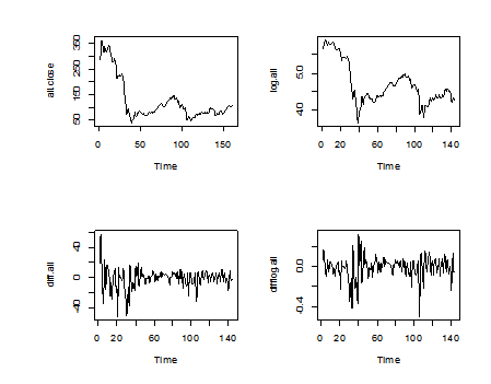
Through comparison, we find percentage change model is much better than differencing of the original data in terms of stationarity.
I have ACF and PACF of the percentage change model:
Picutre 2
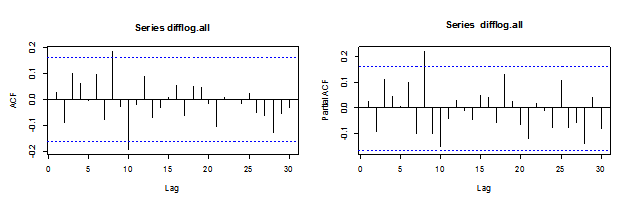
The ACF and PACF cannot help us quickly find the candidates through their movement. Thus I use EACF:
|
AR/MA 0 1 2 3 4 5 6 7 8 9 10 11 12 13 0 o o o o o o o x o x o o o o 1 x o o o o o o o o x o o o o 2 x x o o o o o o o o o o o o 3 x o x o o o o o o o o o o o 4 o o o o o o o o o o o o o o 5 o x x o o o o o o x o o o o 6 x x o o o x o o o x o o o o 7 x x x o o x x o o x o o o o |
Thus I have arima(1,0,1), arima(2,0,2), arima(3,0,3) for candidates selection of percentage change model.
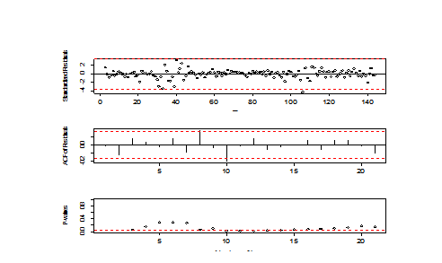
arima(1,1,1)
|
Call: arima(x = log.all, order = c(1, 1, 1)) Coefficients: ar1 ma1 0.8566 -0.8253 s.e. 0.2121 0.2289 sigma^2 estimated as 0.01329: log likelihood = 106.02, aic = -208.04 |
Picture 3
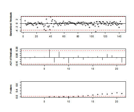
arima(2,1,2)
|
arima(x = log.all, order = c(2, 1, 2)) Coefficients: ar1 ar2 ma1 ma2 -0.3071 -0.9491 0.3787 1.0000 s.e. 0.0342 0.0331 0.0260 0.0322 sigma^2 estimated as 0.01242: log likelihood = 109.13, aic = -210.25 |
Picture 4

arima(3,1,3)
|
Call: arima(x = log.all, order = c(3, 1, 3)) Coefficients: ar1 ar2 ar3 ma1 ma2 ma3 -0.0087 -0.7631 -0.1591 0.0512 0.6876 0.2823 s.e. 0.5256 0.2326 0.4146 0.5106 0.2360 0.3682 sigma^2 estimated as 0.0129: log likelihood = 108.06, aic = -204.12 |
Picture 5

All three tsdiag are bad, thus I choose the model with smallest AIC to fix the model. I observe there are spikes in ACF of the residuals. Thus I add more MA terms. Then I found arima(2,1,4) is one of the best option:
|
arima(x = log.all, order = c(2, 1, 4)) Coefficients: ar1 ar2 ma1 ma2 ma3 ma4 -0.2799 0.5586 0.3560 -0.6776 -0.0009 0.2543 s.e. 0.2865 0.2705 0.2891 0.2963 0.0835 0.0887 sigma^2 estimated as 0.01253: log likelihood = 110.08, aic = -208.16 |
I find ma3 is not significant, thus I remove m3 term. However, the tsdiag is very bad if I remove m3 term. Hence I choose to retain ARIMA(2,1,4), and I call the model is model.x.
The TSDIAG of ARIMA(2,1,3)
Picture 6
Then, I find the residuals of arima(2,1,4) has outliers. I do IO and AO detection.
|
detectIO(mod.4) [,1] [,2] ind 33.000000 106.000000 lambda1 -4.617005 -5.219299 detectAO(mod.4) [,1] [,2] [,3] [,4] ind 31.000000 33.000000 39.000000 106.000000 lambda2 -3.827332 -3.829868 -4.179503 -5.017819 |
Thus I have to add outliers to the model, then I have new model:
|
arima(x = log.all, order = c(2, 1, 4), io = c(31, 33, 39, 106)) Coefficients: ar1 ar2 ma1 ma2 ma3 ma4 IO-31 IO-33 -0.2881 0.2827 0.5190 -0.3318 0.0292 0.3619 -0.1356 -0.3220 s.e. 0.2944 0.3149 0.2789 0.3604 0.1209 0.0817 0.0537 0.0602 IO-39 IO-106 -0.4007 -0.2143 s.e. 0.0575 0.0517 sigma^2 estimated as 0.007312: log likelihood = 148.38, aic = -276.76 |
Then AIC decreases, and diagnosis is very good, and qq-plot is ok.
Picture 7
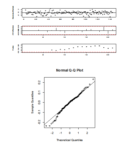
Then I do forecasting with the model. I have the prediction plot(triangular: real values, black dot: forecasting values)
Picture 8
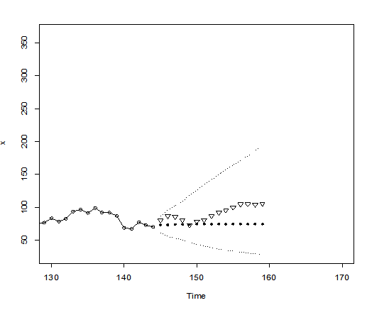
The real values all drop in the 95% confident interval of the prediction. Thus, the model is very good.
I compared predicted values with actual values and forecasting confidence interval. To better demonstrate the effect, relative errors are calculated with the formula, (forecasting-actual)/actual
|
lower upper true prediction relativeerror 1 62.05629 86.76851 80.73 73.37937 -0.09105202 2 56.41439 95.99699 87.43 73.59084 -0.15828846 3 53.65476 102.76531 85.93 74.25529 -0.13586304 4 50.66011 109.63057 80.85 74.52447 -0.07823786 5 46.93304 118.69184 73.11 74.63625 0.02087602 6 44.10548 126.45050 79.11 74.68039 -0.05599308 7 41.41824 134.72294 81.09 74.69931 -0.07880980 8 39.23806 142.23531 87.27 74.70635 -0.14396302 9 37.23555 149.89800 92.59 74.70967 -0.19311294 10 35.51279 157.17404 95.66 74.71070 -0.21899746 11 33.93243 164.49707 99.95 74.71135 -0.25251279 12 32.52290 171.62677 104.80 74.71145 -0.28710446 13 31.22311 178.77220 105.35 74.71160 -0.29082483 14 30.03817 185.82430 104.70 74.71159 -0.28642225 15 28.93846 192.88619 105.95 74.71164 -0.29484061 |
The relative errors are all smaller than 30% from the observation of the table above. Some of the errors are all close to 9%, I think the forecasting is very good.
To better modeling the stock, I will introduce GARCH model. Let us take a look at EACF of │residuals│.
|
AR/MA 0 1 2 3 4 5 6 7 8 9 10 11 12 13 0 o o o o x o o o o o o o o o 1 o o o o o o o o o o o o o o 2 x o o o o o o o o o o o o o 3 x o o o o o o o o o o o o o 4 o o o x o o o o o o o o o o 5 x x x x x o o o o o o o o o 6 x o x o o o o o o o o o o o 7 x x x x o x o o o o o o o o |
Unless we fit a very high order model, it seems that a GARCH(2,2) would be a good choice. Double check for arma structure by looking at ACF of original series:
Picture 9
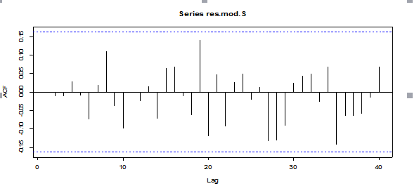
The EACF suggests me use GARCH(1,1). ACF of residuals is very good.
In summary, I elect to first try GARCH(1,1) with t-innovations.
I have the result:
|
garchFit(formula = ~arma(0, 0) + aparch(1, 1), data = res.mod.S, cond.dist = "std", include.mean = FALSE, include.delta = TRUE, leverage = FALSE, trace = FALSE) Error Analysis: Estimate Std. Error t value Pr(>|t|) omega 0.01047 0.01489 0.703 0.482 alpha1 0.09089 0.09419 0.965 0.335 beta1 0.84432 0.16901 4.996 5.86e-07 *** delta 0.85665 4.19154 0.204 0.838 shape 8.38933 6.36267 1.319 0.187 Standardised Residuals Tests: Statistic p-Value Jarque-Bera Test R Chi^2 220.9341 0 Shapiro-Wilk Test R W 0.9202565 3.515701e-07 Ljung-Box Test R Q(10) 6.731871 0.7504922 Ljung-Box Test R Q(15) 9.810444 0.831491 Ljung-Box Test R Q(20) 15.07362 0.7721795 Ljung-Box Test R^2 Q(10) 13.69988 0.1871264 Ljung-Box Test R^2 Q(15) 13.94997 0.529327 Ljung-Box Test R^2 Q(20) 17.17171 0.6417974 LM Arch Test R TR^2 11.25441 0.5072512 |
Now, the model seems ok. Now I check ACF of residuals, and the result look great.
Picture 10

Then I start doing forecasting. I have,
|
meanForecast meanError standardDeviation 1 -1.650886e-04 0.1011043 0.1011043 2 -6.434933e-05 0.1048308 0.1044504 3 -2.668806e-05 0.1077988 0.1073465 4 -1.106853e-05 0.1103419 0.1098650 5 -4.590533e-06 0.1125553 0.1120632 6 -1.903865e-06 0.1144921 0.1139879 7 -7.896037e-07 0.1161920 0.1156773 8 -3.274781e-07 0.1176872 0.1171634 9 -1.358174e-07 0.1190049 0.1184731 10 -5.632852e-08 0.1201677 0.1196289 11 -2.336153e-08 0.1211954 0.1206504 12 -9.688898e-09 0.1221046 0.1215541 13 -4.018347e-09 0.1229098 0.1223544 14 -1.666558e-09 0.1236234 0.1230638 15 -6.911837e-10 0.1242564 0.1236930 |
Then I plug the residual forecast back the arima model. I have new prediction table:
|
true prd abs.errors. 1 80.73 74.37937 0.07866505 2 87.43 74.59084 0.14685074 3 85.93 75.25529 0.12422566 4 80.85 75.52447 0.06586927 5 73.11 75.63625 0.03455404 6 79.11 75.68039 0.04335245 7 81.09 75.69931 0.06647782 8 87.27 75.70635 0.13250433 9 92.59 75.70967 0.18231264 10 95.66 75.71070 0.20854377 11 99.95 75.71135 0.24250779 12 104.80 75.71145 0.27756247 13 105.35 75.71160 0.28133266 14 104.70 75.71159 0.27687115 15 105.95 75.71164 0.28540220 |
lower upper true prediction relativeerror 1 62.05629 86.76851 80.73 73.37937 -0.09105202 2 56.41439 95.99699 87.43 73.59084 -0.15828846 3 53.65476 102.76531 85.93 74.25529 -0.13586304 4 50.66011 109.63057 80.85 74.52447 -0.07823786 5 46.93304 118.69184 73.11 74.63625 0.02087602 6 44.10548 126.45050 79.11 74.68039 -0.05599308 7 41.41824 134.72294 81.09 74.69931 -0.07880980 8 39.23806 142.23531 87.27 74.70635 -0.14396302 9 37.23555 149.89800 92.59 74.70967 -0.19311294 10 35.51279 157.17404 95.66 74.71070 -0.21899746 11 33.93243 164.49707 99.95 74.71135 -0.25251279 12 32.52290 171.62677 104.80 74.71145 -0.28710446 13 31.22311 178.77220 105.35 74.71160 -0.29082483 14 30.03817 185.82430 104.70 74.71159 -0.28642225 15 28.93846 192.88619 105.95 74.71164 -0.29484061 |
The table on the left is the new prediction. And the right one is the old prediction table. Obviously, model with Garch(1,1) is much better in forecasting.
Conclusion and comment:
I have my final model arima(2,1,4)+garch(1,1). It is obviously that he arima(2,1,4)+ garch(1,1) is a better model than ARIMA(2,1,4) for doing prediction. The error ratio is smaller than 30% , and some of them are smaller than 10%. When time increases, the error becomes more inaccurate, and the first couples of prediction are very acurrate. Thus, arima(2,1,4)+ garch(1,1) is a good model for Allianz stock price. To better modeling the stock price, we need large sample size since garch is very greedy to data. I believe with larger sample size, we can have an improved model for forecasting.
Attachment: R-Commander
#define variables
all=read.csv("H:/AZ.csv",header=TRUE)
all.close=all$adjclose
all.close=ts(all.close)
all.int=all.close[1:144]
all.int=ts(all.int)
log.all=log(all.int)
difflog.all=diff(log.all)
#plot of EACF , ACF and PACF
par(mfrow=c(1,2))
acf(difflog.all,lag.max=30);pacf(difflog.all,lag.max=30)
eacf(difflog.all)
#model selection
mod.1=arima(log.all,order=c(1,1,1))
tsdiag(mod.1)
mod.31=arima(log.all,order=c(2,1,2))
tsdiag(mod.31)
mod.6=arima(log.all,order=c(3,1,3))
tsdiag(mod.6)
mod.4=arima(log.all,order=c(2,1,4))
tsdiag(mod.4)
mod.5=arima(log.all,order=c(2,1,3))
tsdiag(mod.5)
mod.7=arima(log.all,order=c(2,1,5))
tsdiag(mod.7)
qqnorm(mod.4$res);qqline(mod.4$res)
mod.10=arima(log.all,order=c(2,1,4),io=c(31,33,39,106))
t=seq(log.all)
p1<-as.numeric(t==31)
p2<-as.numeric(t==33)
p3<-as.numeric(t==39)
p4<-as.numeric(t==106)
S=data.frame(p1,p2,p3,p4)
mod.S=arima(log.all,order=c(2,1,4),xreg=S)
s1<-rep(0,15)
s2<-rep(0,15)
s3<-rep(0,15)
s4<-rep(0,15)
SS<-data.frame(s1,s2,s3,s4)
r=plot(mod.S,n.ahead=15,newxreg=SS,pch=20,xlim=c(130,170))
prediction=r$pred
true=all.close[145:159]
relativeerror=(prediction-true)/true
relativeerror
lower=r$lpi
upper=r$upi
data.frame(lower,upper,true,prediction,relativeerror)
res.mod.S=mod.S$res
eacf(abs(res.mod.S))
acf(res.mod.S,lag.max=40)
res.mod.S=mod.S$res
aparch.1=garchFit(formula=~arma(0,0)+aparch(1,1),data=res.mod.S,cond.dist="std",
include.mean=FALSE,include.delta=TRUE,leverage=FALSE,trace=FALSE)
summary(aparch.1)
acf(aparch.1@residuals)
acf((aparch.1@residuals)^1.423)
#forecasting in Garch
resp=predict(aparch.1,n.ahead=15,transform=exp)
garchpred=resp$meanForecast
prd=garchpred+prediction
errors=(prd-true)/true
data.frame(true,prd,abs(errors))
参考文献:
Data source: http://finance.yahoo.com/q/hp?s=ALV.DE&a=00&b=1&c=2000&d=04&e=1&f=2011&g=m
最新论文
推荐论文
