


 雷达卡
雷达卡


- instrument depvar exogenous = (x4 x5) predetermined = (x6);
instrument depvar exogenous = (x4 x5) predetermined = (x6);
The Arellano and Bond method is very useful in dealing with autoregressive data. It is important to realize, however, that using too many instruments can produce biased parameter estimates and cause computational difficulties since the weighting matrix becomes very large. In Arellano and Bond’s original paper, only the past values of dependent variable are used as instruments. In theory, any variables that are not correlated with the error can be used. However, you have to make sure that the selected instruments are strong and that the model is not misspecified. Inclusion of unnecessary instruments can be partially prevented with the MAXBAND option. Results of the GMM estimation with x4, x5, and x6 specified as exogenous variables are presented in Table 4.
PANEL PROCEDURE AND SAS
The new PANEL procedure enhances the features that were implemented in the TSCSREG procedure. The new methods added include between estimators, pooled estimators, and dynamic panel estimators using GMM. The CLASS statement creates classification variables that are used in the analysis. The FLATDATA statement allows the data to be in a compress form. The TEST statement includes new options for Wald, Lagrange multiplier, and likelihood ratio tests. Since the presence of heteroscedasticity can result in inefficient and biased estimates of the variance covariance matrix in the OLS framework, several methods producing heteroscedasticity-consistent covariance matrices (HCCME) were added. The new RESTRICT statement specifies linear restrictions on the parameters. The PANEL procedure now produces graphical displays by using ODS Graphics. The new plots include residual, predicted, and actual value plots, Q-Q plots, histograms, and profile plots. The OUTPUT statement enables the user to output data and estimates that can be used in other analysis. It is typically difficult to create lagged variables in the panel setting. If lagged variables are created in a DATA step, several programming steps including loops are often needed. The PANEL procedure makes creating lagged values easy by including the LAG statement. The LAG statement, depending on the lag order, can generate a large number of missing values. The PANEL procedure offers a solution to the loss of potentially useful observations by replacing the missing values with zeros, overall mean, time mean, or cross section mean (LAG, ZLAG, XLAG, SLAG, and CLAG statements).
The following SAS statements are used to create lagged values:
- proc panel data=new;
- lag y(1) / out=test;
- id i t;
- run;
proc panel data=new; lag y(1) / out=test; id i t;run;
Even though the new PANEL procedure represents a collection of powerful analytical and visual tools, it is important to remember that other procedures available in SAS/ETS and SAS/STAT software can include models that are not implemented in the PANEL procedure. The LOGISTIC procedure offers fixed-effects models with nonnormal errors in panel setting. The NLMIXED procedure offers an implementation of nonlinear fixed- and random-effects models. The GLIMMIX procedure offers the most complete alternative for both fixed- and random-effects models in linear and nonlinear settings. Other procedures offer the same types of models. For example, it is possible to fit a two-way random-effects model by using the MIXED procedure as follows:
- proc mixed data=two method=type3;
- class i t;
- model y = x1 x2 x3 /solution;
- random i t;
- run;
proc mixed data=two method=type3; class i t; model y = x1 x2 x3 /solution; random i t;run;
The same model can be estimated using the PANEL procedure as follows:
- proc panel data=two;
- model y = x1 x2 x3 / rantwo vcomp = fb;
- id i t;
- run;
proc panel data=two; model y = x1 x2 x3 / rantwo vcomp = fb; id i t;run;
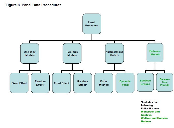
Fixed-effects models are typically easy to implement through the use of dummy variables in many SAS procedures. The random-effects models are more complex and require specialized procedures. Methods available in the PANEL procedure along with a list of procedure handling time series cross-sectional data are depicted in Figure 8. New additions that are available only in the PANEL procedure are shown in green.
CONCLUSION
This paper demonstrated the use of the new PANEL procedure in SAS/ETS software. It used simulated data with known parameter values to show advantages and disadvantages of different methods. Graphical displays produced using ODS Graphics were used to diagnose the fit of different models and correct for data distortion.
It is no surprise that OLS performed relatively poorly, because it ignores the time series cross-sectional nature of data. Using a simulation it was shown that a proper method, including one-way fixed or random effects, can correct for the estimate bias. If heteroscedasticity is present, the PANEL procedure offers several ways to correct for it. If the data are dynamic in nature, the PANEL procedure offers the Arellano and Bond GMM method to regain efficiency. It is important to remember that additional tools not available in the PANEL procedure can be found in other SAS/ETS SAS/STAT procedures. For example, the LOGISTIC procedure offers fixed-effects models with nonnormal errors. Nonlinear models can be estimated using the NLMIXED procedure.

 提升卡
提升卡 置顶卡
置顶卡 沉默卡
沉默卡 变色卡
变色卡 抢沙发
抢沙发 千斤顶
千斤顶 显身卡
显身卡


 京公网安备 11010802022788号


