


 雷达卡
雷达卡


This exercise focuses on linear regression with both analytical (normal equation) and numerical (gradient descent) methods. We will start with linear regression with one variable. From this part of the exercise, we will create plots that help to visualize how gradient descent gets the coefficient of the predictor and the intercept. In the second part, we will implement linear regression with multiple variables. In this part of this exercise, we will implement linear regression with one variable to predict profits for a food truck. Suppose you are the CEO of a restaurant franchise and are considering different cities for opening a new outlet. The chain already has trucks in various cities and you have data for profits and populations from cities. We would like to use this data to help us select which city to expand to next. Load the data and display first 6 observations Before starting on any task, it is often useful to understand the data by visualizing it. For this dataset, we can use a scatter plot to visualize the data, since it has only two properties to plot (profit and population). Many other problems that we encounter in real life are multi-dimensional and can’t be plotted on a 2-d plot. Here it is the plot: In this part, we will fit linear regression parameters θ to our dataset using gradient descent. As we perform gradient descent to learn minimize the cost function J(θ), it is helpful to monitor the convergence by computing the cost. In this section, we will implement a function to calculate J(θ) so we can check the convergence of our gradient descent implementation. The function below calcuates cost based on the equation given above. Now, we can calculate the initial cost by initilizating the initial parameters to 0. Next, we will implement gradient descent by calling the computeCost function above. A good way to verify that gradient descent is working correctly is to look at the value of J(θ) and check that it is decreasing with each step. Our value of J(θ) should never increase, and should converge to a steady value by the end of the algorithm. Now, let’s use the gradientDescent function to find the parameters and we have to make sure that our cost never increases. Let’s use 1500 iterations and a learning rate alpha of 0.04 for now. Later, we will see the effect of these values in our application. We expect that the cost should be decreasing or at least should not be at all increasing if our implementaion is correct. Let’s plot the cost fucntion as a function of number of iterations and make sure our implemenation makes sense. Here it is the plot:本帖隐藏的内容
The file ex1data1.txt contains the dataset for our linear regression problem. The first column is the population of a city and the second column is the profit of a food truck in that city. A negative value for profit indicates a loss. The first column refers to the population size in 10,000s and the second column refers to the profit in $10,000s.
Plotting the Data

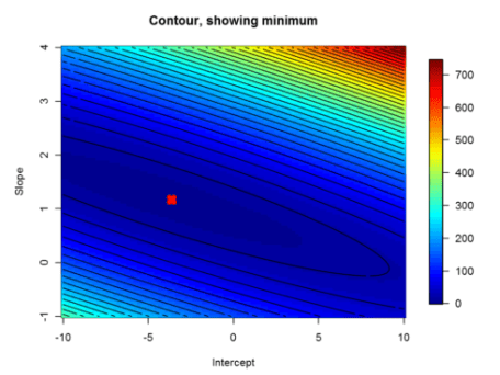
Gradient Descent
To implement gradient descent, we need to calculate the cost, which is given by:

Computing the cost J(θ)
But remember, before we go any further we need to add the θ intercept term.
Gradient descent
The gradient descent function below returns the cost in every iteration and the optimal parameters for the number of iterations and learning rate alpha specified.
Ploting the cost function as a function of the number of iterations

As the plot above shows, the cost decrases with number of iterations and gets almost close to convergence with 1500 iterations.
 提升卡
提升卡 置顶卡
置顶卡 沉默卡
沉默卡 变色卡
变色卡 抢沙发
抢沙发 千斤顶
千斤顶 显身卡
显身卡


 京公网安备 11010802022788号


