论文库 经济学论文 会计学论文 金融学论文 统计学论文 管理学论文 毕业论文 经管之家

Convex Optimization Approach to Solving Nonlinear Regression Models来源：人大经济论坛论文库　作者：Kaiqing Fan　时间：2016-05-26

　　

　　

Convex Optimization Approach to Solving Nonlinear Regression Models

Kaiqing Fan

 

1. Introduction

Picture 4

  

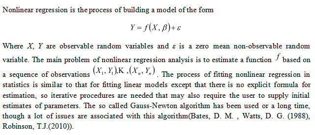
In this project we will go over a convex optimization approach to solving nonlinear regression model proposed by Dimitris Bertsimas,etc(1999). We will also examine this idea by doing a simulation study as well as looking at a case study of decennial U. S. Census population for the United States (in millions), from 1790 through 2000 in the book “An R Companion to Applied Regression, second edition”. For the example, we will compare this idea to the Gauss-Newton method. The software we are going to use are: the cvx package in Matlab and the nls function in R (an environment for statistical computing and graphics, for more information see: http://www.r-project.org/)

 

2. A Convex Optimization Approach to Solving Nonlinear Regression Models

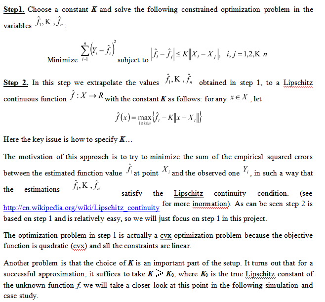
The basic ideas are as follows:

Picture 5

 

3. A Simulation Study

Let us now consider a particular case of a nonlinear model:

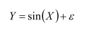
With 0 ≤ X ≤ 2π and noise term ε normally distributed as N(0, σ²). We divide the interval [0, 2π] into n − 1 equal intervals and pick end points of these intervals X_i = 2π(i – 1)/(n – 1), i = 1, 2, …, n.  we generate n independent noise term ε₁, …, ε_n with normal N(0, σ²) distribution. Let n = 50 and σ = 0.5. The above procedure can be implemented in R as follows:

set.seed(123)

ok <- seq(0,1,l = 50)

x <- 2*pi*ok

y <- sin(x)+rnorm(50,0,0.5)

 

Now let K = 1 then K = 2, the proposed convex approach for nonlinear regression can be implemented in Matlab as follows:

 

n = 50;

k = 1

% k = 2

x = [0.0000000; …; 6.2831853];

y = [-0.280237823;  …; -0.041684533];

cvx_begin

    variables f(n)

    minimize norm(y - f)

for i = 1 : n,

  for j = 1:n,

    abs(f(i) - f(j)) <= k*norm(x(i) - x(j));

  end

end

cvx_end

 

The generated data and the fitted curves for K = 1 then K = 2 are plotted below:

Picture 1

 

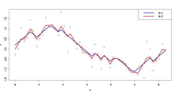
We see that the algorithm is successful in obtaining a fairly close approximation of the function sin(x). So the simulation study shows that our approach works very well. Now let’s look at a case study…

 

 

4. A Case Study

As a case study, let us consider the data frame USPop in the car package of R, which has decennial U. S. Census population for the United States (in millions), from 1790 through 2000. The data are shown in Figure below (a):

Picture 2

 

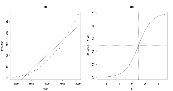
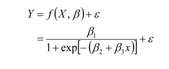
The simple linear regression least-squares line shown on the graph clearly does not match these data: The U. S. population is not growing by the same rate in each decade, as is required by the straight-line model. A common simple model for population growth is the logistic growth model,

Picture 6

A prototype of this function is shown in the above picture (b).

In statistics the above model can be fitted in R as follows:

pop.mod <- nls(population ~ beta1/(1 + exp(-(beta2 + beta3*year))),

start=list(beta1 = 400, beta2 = -49, beta3 = 0.025),

data=USPop, trace=TRUE)

ff <-fitted(pop.mod)

lines(ff ~ USPop$year)

 

Note here we use nls function in R to do this job. To apply this function we have to guess the initial values for the parameters, which in my opinion, is the down side of this method. Also the default estimation method is the so called Gauss-Newton method. Honestly speaking, this approach works well...the results are plotted on page 6.

Now let’s look at our approach. This can be implemented in Matklab as follows:

n = 22;

k = 1

%k = 2

% k = 3

x = [1790 1800 1810 1820 1830 1840 1850 1860 1870 1880 1890 1900 1910 1920 1930 1940 1950 1960 1970 1980 1990 2000]';

y = [3.929214 5.308483 7.239881 9.638453 12.860702 17.063353 23.191876 31.443321 38.558371 50.189209 62.979766 76.212168 92.228496 106.021537 123.202624 132.164569 151.325798 179.323175 203.302031 226.542199 248.709873 281.421906]';

cvx_begin

    variables f(n)

    minimize norm(y - f)

for i = 1 : n,

  for j = 1:n,

    abs(f(i) - f(j)) <= 2.5*norm(x(i) - x(j));

  end

end

cvx_end

 

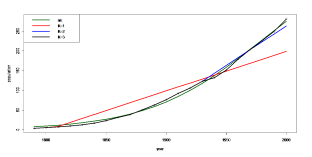
Here we choose to use K = 1 then K = 2 and then K = 3. We will plot the result together to select the best one.

The Figure on page 6 represents the results from nls approach and cvx approach with above 3 K values. It can be seen that the nls approach just give us a smoothed curve. While the cvx approach with the piecewise linear curve can fit any fluctuates in the original data. Actually in this case when K = 3 we got a perfectly model…

Picture 3

 

5. A Concluding Remark

We have examined a convex optimization approach to the nonparametric regression estimation problem. Since it is nonparametric, so the fitted model is not a smoothed curve but piecewise linear curves. So if one does not want assume for the underlying distribution of the data, and then this would be a very good approach. As long as we can pick up an appropriate K value, we can actually model the data perfectly…

 

References:

• Dimitris Bertsimas,etc(1999), Estimation of Time-Varying Parameters in Statistical Models: an Optimization Approach, Machine Learning 35, 225–245

• Bates, D. M. , Watts, D. G. (1988), Nonlinear Regression Analysis and Its Applications, Wiley

• John Fox, Sanford Weisberg, Nonlinear Regression and Nonlinear Least Squares in R --- An Appendix to An R Companion to Applied Regression, second edition, 2010

参考文献：
　　 References: • Dimitris Bertsimas,etc(1999), Estimation of Time-Varying Parameters in Statistical Models: an Optimization Approach, Machine Learning 35, 225–245 • Bates, D. M. , Watts,