论文库 经济学论文 会计学论文 金融学论文 统计学论文 管理学论文 毕业论文 经管之家

Short-Term Forecast of Foreign Exchange Reserves using Time Serize Analysis with R来源：人大经济论坛论文库　作者：Kaiqing Fan　时间：2016-05-25

Short-Term Forecast of the Monthly Foreign Exchange Reserves

(From 1/2011 to 1/2012)

Kaiqing Fan

Data description:

The monthly foreign exchange reserves for China has been kept going up from 1978, but the available time series data I can find online is only from December 1999. At the end of 1999, Chinese Government decided to improve the number of foreign exchange reserves to prevent the international financial and economic risks. From that time on, the reserves have gone up very quickly. In December 1999, Chinese foreign exchange reserves is only 1546.75 (unit: 100 million US dollars), at the end of 2010, the reserves reached at 28473.38 million US dollars. I choose the monthly foreign exchange reserves for Chinese Government from December 1999 to December 2010 to do time series analysis.

Resource:

http://www.safe.gov.cn/  ,there is an English version in this website.

Introduction

To apply for entering World Trade Organization, Chinese Government adjusted her policies to prepare this application. One of these adjustments was to improve the foreign exchange reserves against the international economic and financial risks. So from December 1999 on, China’s foreign exchange reserves has been going up. From 2004 on, Chinese Government adjusted her policies to appreciate the value of RMB---Chinese dollar by small amplitude, a safe and healthy, and under control steps, lots of US dollars entered into China to arbitrage, this speeded up the accumulation of China’s foreign.

Analysis of the Original Data

library(TSA)

x=scan(file.choose()) ; y=ts(x)

plot(y)

acf(y)

pacf(y)

Pic 1

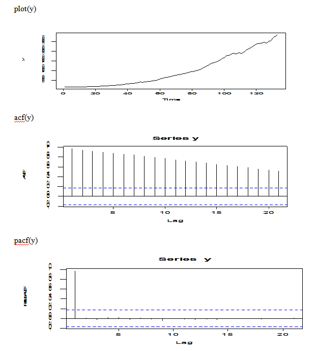
From the plot of original data, we may try to do some transformation because the original data is non-stationary and the plot shows increasing trend. From the ACF(y), there is an exp decay, but the plot is dying of very slowly; From the PACF(y), there is 0 for k>1.

Transformations and Candidate Model Identifying

plot(log(y))

Pic 2

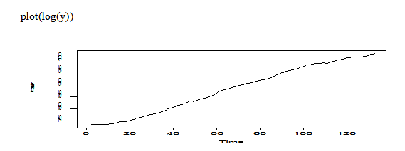
The transformation of log original data still shows trend, non-stationary.

plot(diff(y))

Pic 3

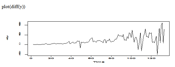
ff=diff(x)

adf.test(ff)

Augmented Dickey-Fuller Test

data:  ff

Dickey-Fuller = -3.0121, Lag order = 5, p-value = 0.1544

alternative hypothesis: stationary

The transformation of difference on original data still shows non-stationary. Let’s try difference of log original data.

plot(diff(log(y)))

Pic 4

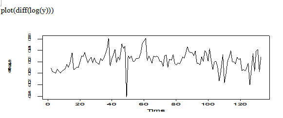
fan=diff(log(y))

adf.test(fan)

  Augmented Dickey-Fuller Test

data:  fan

Dickey-Fuller = -3.4266, Lag order = 5, p-value = 0.05267

alternative hypothesis: stationary

The transformation of diff(log(fan)) is not too bad, we can think it is stationary.

acf(diff(log(y)))

pacf(diff(log(y)))

Pic 5

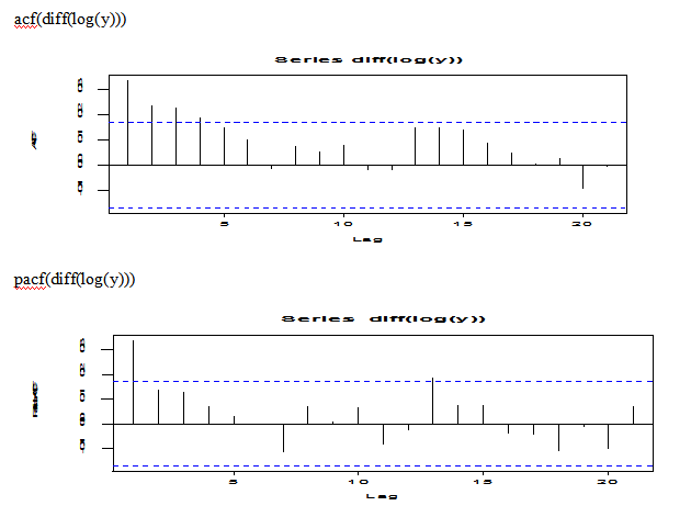
The plot of diff(log(y)) looks no trend; the plot of ACF(diff(log(y))) shows some form exp decay; the plot of PACF(diff(log(y))) shows 1 spike. So we may try AR(1) model for the diff(log(y)) transformation.

But this is not much help, we may try looking at EACF.

eacf(diff(log(y)))

AR/MA

   0 1 2 3 4 5 6 7 8 9 10 11 12 13

0 x x x x o o o o o o o  o  o  o

1 x o o o o o o o o o o  o  o  o

2 x x o o o o o o o o o  o  o  o

3 x o o o o o o o o o o  o  o  o

4 x o o o o o o o o o o  o  o  o

5 x o o o o o o o o o o  o  o  o

6 o x x o o o o o o o o  o  o  o

7 x x x o x o o o o o o  o  o  o

Let’s try ARMA(1,1), MA(4) model for this diff(log(y)) transformation.

Model Selection by AIC, AICc, BIC and their Coefficients

MA(4) model for diff(log(y))

fan=diff(log(y))

arima(fan,order=c(0,0,4))

Call: arima(x = fan, order = c(0, 0, 4))

Coefficients:           ma1     ma2     ma3     ma4  intercept

                             0.2551  0.1246  0.1788  0.1482     0.0220

                     s.e.  0.0868  0.0876  0.0872  0.0870     0.0021

sigma^2 estimated as 0.0002006:  log likelihood = 374.53,  aic = -739.06

IC=function(AIC,n,k){

AICc=AIC+2*k*(k+1)/(n-k-1)

BIC=AIC-2*k+log(n)*k

return(list(c("AIC=",AIC),c("AICc=",AICc),c("BIC=",BIC)))

}

IC(-739.06,length(fan),9)

 [1] "AIC="    "-739.06"

 [1] "AICc="             "-737.584590163934"

 [1] "BIC="              "-713.114782696723"

ARMA(1,1) Model for diff(log(y))

arima(fan, order=c(1,0,1))

Call: arima(x = fan, order = c(1, 0, 1))

Coefficients:           ar1      ma1  intercept

                            0.8180  -0.5746     0.0217

                      s.e.  0.1177   0.1667     0.0028

sigma^2 estimated as 0.0001985:  log likelihood = 375.2,  aic = -744.41

IC(-744.41,length(fan),9)

 [1] "AIC="    "-744.41"

 [1] "AICc="             "-742.934590163934"

 [1] "BIC="              "-718.464782696723"

AR(1) Model for diff(log(y))

> arima(fan, order=c(1,0,0))

Call: arima(x = fan, order = c(1, 0, 0))

Coefficients:            ar1  intercept

                           0.3364     0.0220

                    s.e.  0.0818     0.0019

sigma^2 estimated as 0.0002069:  log likelihood = 372.52,  aic = -741.05

 IC(-741.05,length(fan),9)

 [1] "AIC="    "-741.05"

 [1] "AICc="             "-739.574590163934"

 [1] "BIC="              "-715.104782696723"

Summary of the Comparisons Among the Three Candidate Models For diff(log(y))

For MA(4) model, we can see that its AIC, AICc, BIC are the largest among the three candidate models, and its coefficients of ma2, ma3 and ma4 are borderline;

For ARMA(1,1) model, its AIC, AICc, BIC are the smallest among the three candidate models, and its coefficients are all OK;

For AR(1) model, its AIC, AICc, BIC are the 2^nd smallest among the three candidate models, but its coefficient of ar1, ar3 is pretty good;

So we choose ARMA(1,1) as the best model.

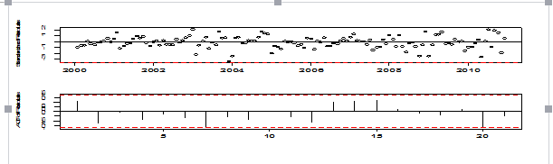
Diagnosis for ARMA(1,1) model of diff(log(y))

mod1=arima(fan, order=c(1,0,1))

tsdiag(mod1)

Pic 6

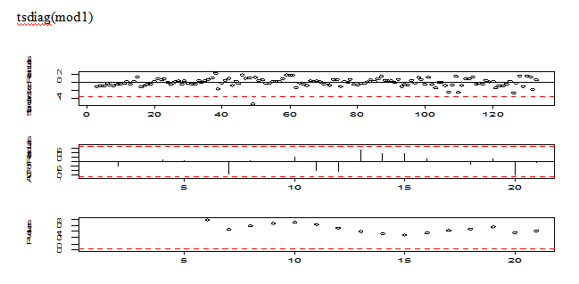
The stardandized residuals looks like randomly distributed, but there is one outliers located at around the 50^th position; the residual autocorrections look excellent; the plot of p-values are all non-significant.

qqnorm(mod1$residuals)

abline(mean(mod1$residuals),sd(mod1$residuals))

Pic 7

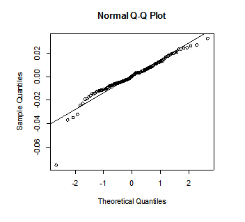
QQ plot for normality shows there may one outliers at the left bottom corner, this outlier violates the assumptions of the white noise. We should handle with this potent outlier in the coming future.

res=rstandard(mod1)

plot(res,ylab='ARMA(1,1), residuals')

abline(h=0)

Pic 8

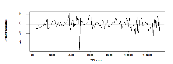
If we ignore the point located at around time 50,then the plot of ARMA(1,1) for residuals for diff(log(y)) looks good, there is no trend.

All in all, the model ARMA(1,1) is not as perfect as we expected because of the outlier, we need to deal with it.

Test for outliers and refit the ARMA(1,1) model

detectAO(mod1)

             [,1]

ind     48.000000

lambda2 -6.030457

Let’s refit the ARMA(1,1) model incorporating an AO outlier at time t=48. ( t=48 here because this data is diff(log(y)))

If I don’t take differencing, then the outlier would be t-=49, let’s see the following:

library(TSA)

originalx=scan(file.choose())

y=ts(originalx)

y133=window(y, end=133)

rey=ts(y133,start=c(1999,12),frequency=12)

mod1=arima(x=log(rey), order=c(1,1,1),xreg=seq(1,length(rey)))

Call: arima(x = log(rey), order = c(1, 1, 1), xreg = seq(1, length(rey)))

Coefficients:         ar1      ma1    xreg

                          0.8183  -0.5750  0.0217

                  s.e.  0.1176   0.1666  0.0028

sigma^2 estimated as 0.0001985:  log likelihood = 375.2,  aic = -744.41

detectAO(mod1)

             [,1]

ind     49.000000

lambda2 -6.043367

tg=seq(rey)

AO49=as.numeric(tg==49)

mod2<-arimax(log(rey),xreg=data.frame(tg,AO49),order=c(1,1,1) xreg = data.frame(tg, AO49))

Call: arimax(x = log(rey), order = c(1, 1, 1), xreg = data.frame(tg, AO49))

Coefficients:           ar1      ma1      tg     AO49

                       0.9772  -0.6707  0.0445  -0.0370

                s.e.     NaN   0.0989     NaN   0.0088

sigma^2 estimated as 0.0001834:  log likelihood = 379.78,  aic = -751.56

Warning message: In sqrt(diag(x$var.coef)) : NaNs produced

tsdiag(mod2)

Pic 9

Looks like mod2 is not a good model because of R package crushed. We may think of the second best model ARIMA(1,1,0), i.e., AR(1) model on diff(log(rey)).

Let’s try to Test for outliers and refit the ARIMA(1,1,0) model

mod3=arima(x=log(rey),order=c(1,1,0),xreg=seq(1,length(rey)))

Call: arima(x = log(rey), order = c(1, 1, 0), xreg = seq(1, length(rey)))

Coefficients:          ar1    xreg

                            0.3364  0.0220

                     s.e.  0.0818  0.0019

sigma^2 estimated as 0.0002069:  log likelihood = 372.52,  aic = -741.05

tsdiag(mod3)

Pic 10

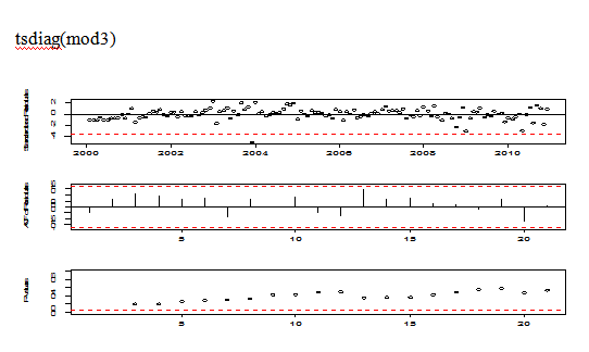
The plot of diagnosis is good except for an outlier at around t=49.

qqnorm(mod3$residuals)

abline(mean(mod3$residuals),sd(mod3$residuals))

Pic 11

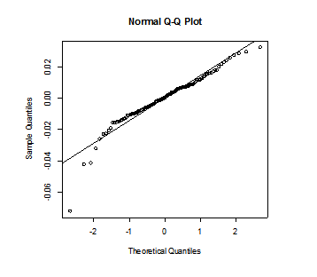
QQ plot looks not so nice because of outlier.

detectAO(mod3)

             [,1]

ind     49.000000

lambda2 -5.924306

detectIO(mod3)

             [,1]

ind     49.000000

lambda1 -5.487006

tg=seq(rey)

AO49=as.numeric(tg==49)

mod4<-arimax(log(rey),xreg=data.frame(tg,AO49),order=c(1,1,0))

Call: arimax(x = log(rey), order = c(1, 1, 0), xreg = data.frame(tg, AO49))

Coefficients:          ar1      tg     AO49

                           0.4428  0.0223  -0.0389---are very small, non-significant.

                        s.e.  0.0779  0.0020   0.0079

sigma^2 estimated as 0.0001719:  log likelihood = 384.7,  aic = -763.41

The coefficients of AO49 and tg are all non-significant, so we can ignore tg and AO49 terms,then I do not want to use ARIMA(1,1,0) with AO49 to do forecasting.

So I still choose the model ARIMA(1,1,1) without AO49 to do forecasting.

Rethink the outlier at the 49th position

Let’s take a look at part of the log(rey) and part of original data.

When we compare the log(rey) values and the real values , we can see that the 49^th position is December 2003,its value is 8.302144 , its real number is 4032.51;in November 2003, it is 8.343699,the real number is 4203.61; in January 2004, it is 8.332597, its real number is 4157.20.  They don’t differentiate too much.

The reasons for the decreasing of US dollars on China’s foreign exchange reserves in December 2003 were that the value of US dollars fell after 2003, China’s foreign exchange reserves in the book were serious devaluation, a loss of about $ 200 billion in the end of 2003. We can think we should keep this outlier in out model, because the depreciation and appreciation of international monetary always happen.    

So I may keep this outlier at t=49, then use mod1 ARIMA(1,1,1)to do further forecasting.

Forecasting using mod1 ARIMA(1,1,1)

n=length(rey); lead=13

new.t=seq(n+1,n+lead)

plot(mod1,n.ahead=lead,newxreg=new.t,ylab='Log(China foreign exchange reserves)', xlab='Month',n1=2006, pch=19)

Pic 12

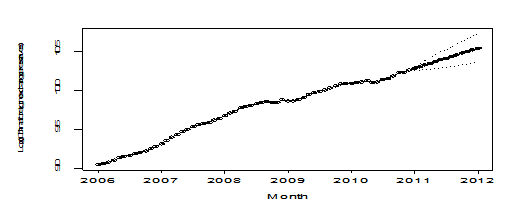
The plot of forecast looks very nice.

result=plot(mod1,n.ahead=lead,newxreg=new.t,ylab='China foreign exchange reserves', xlab='Month', transform=exp, pch=19,n1=2006, lty=1,type='o')

points(new.t[134:146], rey[134:146], pch=6)

Pic 13

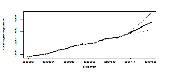
The plot of forecast looks very nice.

forecast=result$pred

actual=y[134:146]

lower=result$lpi

upper=result$upi

cbind(lower,forecast,actual,upper)

month	year	lower	forecast	acutal	upper
Jan	2011	28322.46	29115.53	29316.74	29930.8
Feb	2011	28485.69	29768.92	29913.86	31109.96
Mar	2011	28679.17	30434.27	30446.74	32296.79
Apr	2011	28889.65	31112.23	31458.43	33505.8
May	2011	29115.3	31803.4	31659.97	34739.67
Jun	2011	29356.27	32508.33	31974.91	35998.83
Jul	2011	29613.03	33227.56	32452.83	37283.28
Aug	2011	29885.92	33961.6	32624.99	38593.11
Sep	2011	30175.09	34710.93	32016.83	39928.6
Oct	2011	30480.55	35476.02	32737.96	41290.2
Nov	2011	30802.19	36257.32	32209.07	42678.57
Dec	2011	31139.84	37055.29	31811.48	44094.45
Jan	2012	31493.28	37870.36	上一篇：【数据挖掘算法工程师】国内某上市企业聘 下一篇：Statistical prediction of EI Nino and Hurricanes 相关论文 【数据挖掘算法工程师】国内某上市企业聘 招聘【数据挖掘算法工程师】 数据挖掘技术及其应用的实现 论精密工程测量及其应用 关于现代机械设计技术的分析 建筑工程施工机械安全管理研究 社会统计结论中存在的一些解释性矛盾问题透析 社会统计结论中存在的一些解释性矛盾问题透析 Using GEE Methodology to Compare Two Treatments for a Respiratory Disorder using SAS Statistical prediction of EI Nino and Hurricanes Short Term forecasting Stock Prize using Time Series Analysis Statistical Estimatation the damage Insurance Company Should Pay Convex Optimization Approach to Solving Nonlinear Regression Models Using Gee Method to analyze whether Church Life Affects Life Expectation 关键词标签 科技进步与对策 经济问题探索 布朗运动 科技管理研究 科学计数法 方差公式 回归分析 主成分分析 可信区间 净资产 开题报告 注册税务师 协方差 标准差 马太效应 最小二乘法 资产负债率 谷歌学术 谷粉学术 实变函数与泛函分析 学者专题 李龙飞 刘遵义 邹至庄 刘大中 李红昌 林晓言 李卫东 李雪梅 Howard 高宏伟 郭丽华 冯华 曹志刚 陈佩虹 卜伟 林海芬 陈艳 冯巧根 徐斌 贾凡胜 最新论文 [审计学]　新会计制度对财务管理的影响 [统计分析]　Journal of Statistical Softwar ... [本科论文]　试分析萨满神画工艺美术创作的意 ... [统计分析]　通过企业经济统计学提高企业经济 ... [统计分析]　高校经济管理类专业统计学教学反 ... [统计分析]　统计学在金融领域的应用 [统计分析]　统计学教学内容及实训的思考 [统计分析]　数理统计学的历史演进 [统计分析]　经济统计学专业建设研究 [统计分析]　大数据与统计学协同发展的思考分 ... 推荐论文 [企业管理]ERP沙盘模拟实验报告 [本科论文]　“一带一路”连通“中国梦”与“ ... [微观经济学]　微观经济学论文 [管理学论文]　浅谈企业战略管理 [公共管理]　当前我国贫富差距问题的现状、原 ... [企业管理]　用友ERP沙盘企业经营模拟战术分析 ... [风险管理]　浅谈小微企业贷款的风险与防范 [微观经济学]　从微观经济学角度分析影响房价的 ... [银行管理]　互联网金融冲击下传统商业银行的 ... [管理学论文]　人力资源毕业论文范文 关于我们 手机版 举报 联系我们 招聘英才 010-80442101 为做大做强论坛，本站接受风险投资商咨询，请联系（010-62719935） 京ICP备11001960号 京ICP证090565号 京公网安备1101084107号 论坛法律顾问：王进律师 知识产权保护声明 免责及隐私声明 MSN：pinggu.org@hotmail.com 邮箱：service@pinggu.org 合作咨询电话：(010)62719935 广告合作电话： 13661292478 （刘老师） 投诉电话：(010)68466864 不良信息处理电话：13661292478