遗传算法优化编码序列实现编码超表面RCS缩减

是 否 +2 论坛币

k人 参与回答

经管之家送您一份

应届毕业生专属福利!

求职就业群

赵安豆老师微信：zhaoandou666

经管之家联合CDA

送您一个全额奖学金名额~ !

立即领取

感谢您参与论坛问题回答

经管之家送您两个论坛币！

+2 论坛币

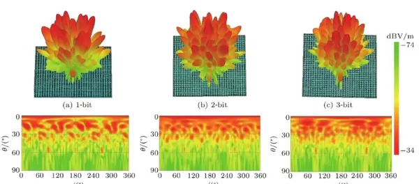
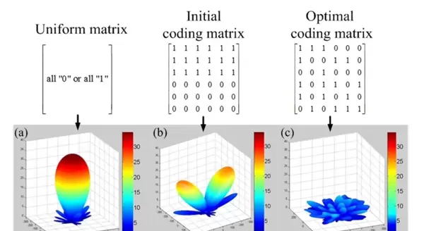
在天线与雷达隐身技术的研究中，编码超表面的雷达散射截面积（RCS）缩减已成为一个关键方向。通过引入遗传算法对编码序列进行优化，可显著提升漫反射性能，从而有效降低目标被探测的概率。该方法兼容多种位数（如1bit、2bit、3bit等）及不同规模（如6×6、8×8等）的编码阵列设计，并具备对单元相位偏差的容差能力，增强了工程实现的可行性。

利用MATLAB或Python编写相应代码，能够快速完成编码序列的优化过程，并自动生成远场分布结果。通过叠加公式计算远场波形，可直观观察优化后的电磁响应特性。同时，结合CST仿真软件，可以进一步验证超表面在实际电磁环境下的RCS缩减效果。

遗传算法的基本原理

遗传算法是一种模拟生物进化机制的全局优化方法，基于选择、交叉和变异操作，在迭代过程中不断筛选出适应度更高的个体。在此应用中，每个个体代表一种可能的编码序列，而适应度函数则依据其对应的RCS表现或漫反射均匀性来定义——RCS越低，适应度越高，优化目标即为寻找最优编码排布。

MATLAB中的实现流程

编码序列初始化

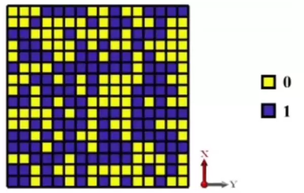
使用MATLAB生成初始种群，通常设定种群大小为50，每个个体为6×6尺寸的2bit编码矩阵。通过随机整数生成函数，确保每个元素落在0到2^num_bits - 1范围内，完成多样化的初始布局构建。

% 以6*6的2bit编码序列为例
num_rows = 6;
num_cols = 6;
num_bits = 2;
pop_size = 50; % 种群大小
population = randi([0, 2^num_bits - 1], [num_rows, num_cols, pop_size]);

randi

适应度评估

定义calculate_fitness函数用于量化每个个体的性能表现。遍历当前种群，调用预设的RCS计算模块（需用户自定义，示例中已简化处理），获取对应电磁响应值，并以RCS的倒数作为适应度指标——数值越大表示性能越优。

function fitness = calculate_fitness(population)
    % 这里假设我们有一个计算RCS的函数calculate_RCS
    [num_rows, num_cols, pop_size] = size(population);
    fitness = zeros(1, pop_size);
    for i = 1:pop_size
        individual = population(:, :, i);
        fitness(i) = calculate_RCS(individual);
    end
    % 这里RCS越小，适应度越高，所以取倒数作为适应度
    fitness = 1./ fitness; 
end

calculate

RCS

遗传操作执行

包括三大核心步骤：

• 选择：依据适应度高低挑选优质父代个体；
• 交叉：随机选取交叉点，将两个父代的部分编码片段重组，生成新后代；
• 变异：按设定概率对某些编码位进行随机翻转，增加种群多样性。

% 选择操作
function selected_population = selection(population, fitness, num_parents)
    [~, idx] = sort(fitness, 'descend');
    selected_population = population(:, :, idx(1:num_parents));
end

% 交叉操作
function new_population = crossover(parents, num_offspring)
    [num_rows, num_cols, num_parents] = size(parents);
    new_population = zeros(num_rows, num_cols, num_offspring);
    for i = 1:num_offspring
        parent1_idx = randi(num_parents);
        parent2_idx = randi(num_parents);
        parent1 = parents(:, :, parent1_idx);
        parent2 = parents(:, :, parent2_idx);
        crossover_point = randi([1, num_rows - 1]);
        new_population(1:crossover_point, :, i) = parent1(1:crossover_point, :);
        new_population(crossover_point + 1:end, :, i) = parent2(crossover_point + 1:end, :);
    end
end

% 变异操作
function mutated_population = mutation(population, mutation_rate)
    [num_rows, num_cols, pop_size] = size(population);
    mutated_population = population;
    for i = 1:pop_size
        for j = 1:num_rows
            for k = 1:num_cols
                if rand < mutation_rate
                    mutated_population(j, k, i) = randi([0, 2^num_bits - 1]);
                end
            end
        end
    end
end

主循环与结果输出

设置最大进化代数，每一代依次执行适应度计算与遗传操作，持续追踪最优解的变化趋势。最终输出收敛后的最佳编码序列，可用于后续仿真分析。

num_generations = 100;
num_parents = 20;
mutation_rate = 0.01;
for generation = 1:num_generations
    fitness = calculate_fitness(population);
    parents = selection(population, fitness, num_parents);
    offspring = crossover(parents, pop_size - num_parents);
    new_population = mutation([parents, offspring], mutation_rate);
    population = new_population;
end
best_individual_idx = find(fitness == max(fitness));
best_individual = population(:, :, best_individual_idx);

Python中的实现方式

种群初始化

借助NumPy库完成编码矩阵的随机生成，结构与MATLAB一致，构建由多个6×6二维数组组成的种群，支持灵活调整位深度与阵列规模。

import numpy as np

num_rows = 6
num_cols = 6
num_bits = 2
pop_size = 50
population = np.random.randint(0, 2**num_bits, size=(num_rows, num_cols, pop_size))

numpy

适应度函数设计

Python版本同样采用RCS倒数作为适应度标准，调用外部仿真接口或近似模型获取个体性能数据，保持与MATLAB逻辑的一致性。

def calculate_fitness(population):
    num_rows, num_cols, pop_size = population.shape
    fitness = np.zeros(pop_size)
    for i in range(pop_size):
        individual = population[:, :, i]
        # 假设calculate_RCS函数已定义
        fitness[i] = calculate_RCS(individual)
    fitness = 1 / fitness
    return fitness

calculate_RCS

遗传算子实现

利用Python内置的random模块或NumPy实现选择、交叉与变异过程，操作方式与MATLAB相似，但语法更简洁，便于调试与扩展。

import random


def selection(population, fitness, num_parents):
    sorted_idx = np.argsort(fitness)[::-1]
    selected_population = population[:, :, sorted_idx[:num_parents]]
    return selected_population


def crossover(parents, num_offspring):
    num_rows, num_cols, num_parents = parents.shape
    new_population = np.zeros((num_rows, num_cols, num_offspring))
    for i in range(num_offspring):
        parent1_idx = random.randint(0, num_parents - 1)
        parent2_idx = random.randint(0, num_parents - 1)
        parent1 = parents[:, :, parent1_idx]
        parent2 = parents[:, :, parent2_idx]
        crossover_point = random.randint(1, num_rows - 1)
        new_population[0:crossover_point, :, i] = parent1[0:crossover_point, :]
        new_population[crossover_point:, :, i] = parent2[crossover_point:, :]
    return new_population


def mutation(population, mutation_rate):
    num_rows, num_cols, pop_size = population.shape
    mutated_population = population.copy()
    for i in range(pop_size):
        for j in range(num_rows):
            for k in range(num_cols):
                if random.random() < mutation_rate:
                    mutated_population[j, k, i] = random.randint(0, 2 ** num_bits - 1)
    return mutated_population

random

主循环结构

循环控制机制与MATLAB类似，逐代演化并记录每代最优个体，直至达到预设终止条件，输出最终优化结果。

num_generations = 100
num_parents = 20
mutation_rate = 0.01
for generation in range(num_generations):
    fitness = calculate_fitness(population)
    parents = selection(population, fitness, num_parents)
    offspring = crossover(parents, pop_size - num_parents)
    new_population = mutation(np.concatenate((parents, offspring), axis=2), mutation_rate)
    population = new_population

best_individual_idx = np.argmax(fitness)
best_individual = population[:, :, best_individual_idx]

远场仿真可视化代码

MATLAB绘图功能

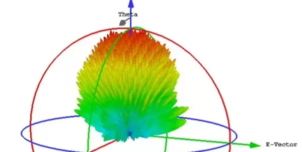
使用MATLAB内置的三维绘图函数，如surf或专用电磁场可视化工具，绘制远场辐射模式的立体图像；同时调用二维绘图命令展示能量分布图，清晰呈现漫反射效果。

% 假设已经得到最佳编码序列best_individual
% 计算远场效果（这里假设已有计算远场的函数calculate_far_field）
far_field_result = calculate_far_field(best_individual);

% 三维仿真
figure;
surf(far_field_result);
title('三维远场效果');
xlabel('X方向');
ylabel('Y方向');
zlabel('幅度');

% 二维能量图
figure;
contourf(abs(far_field_result));
title('二维能量图');
xlabel('X方向');
ylabel('Y方向');

surf

contourf

Python绘图实现

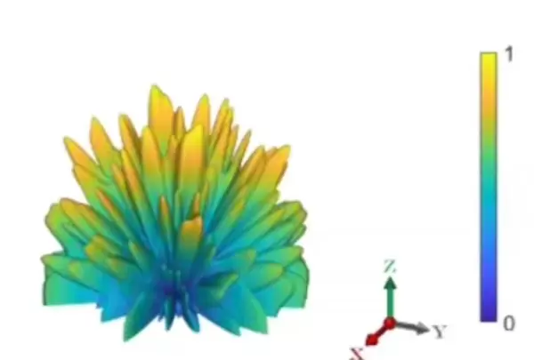
借助Matplotlib与Mayavi等可视化库，Python同样可实现高质量的三维远场仿真图与二维能量分布图，图形风格可定制，适合科研报告与论文插图需求。

import matplotlib.pyplot as plt
import numpy as np

# 假设已经得到最佳编码序列best_individual
# 计算远场效果（这里假设已有计算远场的函数calculate_far_field）
far_field_result = calculate_far_field(best_individual)

# 三维仿真
fig = plt.figure()
ax = fig.add_subplot(111, projection='3d')
X, Y = np.meshgrid(np.arange(far_field_result.shape[0]), np.arange(far_field_result.shape[1]))
ax.plot_surface(X, Y, np.abs(far_field_result), cmap='viridis')
ax.set_title('三维远场效果')
ax.set_xlabel('X方向')
ax.set_ylabel('Y方向')
ax.set_zlabel('幅度')

# 二维能量图
plt.figure()
plt.contourf(np.abs(far_field_result), cmap='viridis')
plt.title('二维能量图')
plt.xlabel('X方向')
plt.ylabel('Y方向')
plt.colorbar()
plt.show()

matplotlib

CST中查看RCS缩减效果的操作步骤

模型建立： 在CST Studio Suite中搭建超表面几何结构，根据优化所得编码序列配置各个单元的状态，确保排列顺序与尺寸符合设计要求。

求解器设置： 选用合适的求解器类型（如时域求解器或频域求解器），设定工作频率范围、边界条件、激励源以及网格划分精度，保证仿真准确性。

结果分析： 仿真完成后，在后处理模块中提取RCS相关数据，绘制其随入射角度或频率变化的曲线图，直观对比优化前后RCS差异，验证缩减效果。

综上所述，通过遗传算法对编码序列进行智能优化，结合MATLAB与Python编程实现高效求解，再辅以CST的高精度电磁仿真，能够系统化地达成编码超表面的RCS抑制目标。该方案不仅适用于多种bit数和阵列规模，还考虑了实际加工中可能出现的相位误差，具备较强的鲁棒性和实用价值，在现代隐身技术和高性能天线设计中具有广阔的应用前景。

扫码加我 拉你入群

请注明：姓名-公司-职位

以便审核进群资格，未注明则拒绝

分享0 收藏0 回帖

关键词：遗传算法优化 遗传算法 Generations concatenate Population