第1章 机器学习基础

是 否 +2 论坛币

k人 参与回答

经管之家送您一份

应届毕业生专属福利!

求职就业群

赵安豆老师微信：zhaoandou666

经管之家联合CDA

送您一个全额奖学金名额~ !

立即领取

感谢您参与论坛问题回答

经管之家送您两个论坛币！

+2 论坛币

1.1 案例学习

作为人工智能的关键组成部分，机器学习正在重塑我们解决各种问题的方式。在这一部分，我们将通过一个具体的例子来深入了解机器学习的工作流程及其核心概念。

房价预测案例

设想我们需要建立一个模型来预测房产的价格。这属于一个回归问题，我们的目标是基于房产的不同属性（例如面积、卧室数量、地理位置等）来预测其市场价值。

问题分析：

• 输入特征：房产面积、卧室数量、房产年龄、地理位置等
• 输出目标：房产价格
• 任务类型：监督学习中的回归问题

接下来，我们将通过Python编程语言来实现这一案例：

import numpy as np
import matplotlib.pyplot as plt
from sklearn.linear_model import LinearRegression
from sklearn.model_selection import train_test_split
from sklearn.metrics import mean_squared_error, r2_score
import pandas as pd

# 生成模拟的房价数据
np.random.seed(42)
num_samples = 200

# 房屋面积（平方米）
area = np.random.normal(120, 40, num_samples)
area = np.clip(area, 50, 250)  # 限制在50-250平方米之间

# 卧室数量
bedrooms = np.random.choice([1, 2, 3, 4, 5], num_samples, p=[0.1, 0.2, 0.4, 0.2, 0.1])

# 房龄（年）
age = np.random.exponential(15, num_samples)
age = np.clip(age, 0, 50)  # 限制在0-50年之间

# 生成房价（万元），基于公式：价格 = 1.5*面积 + 20*卧室 - 1*房龄 + 噪声
price = 1.5 * area + 20 * bedrooms - 1 * age + np.random.normal(0, 30, num_samples)
price = np.clip(price, 100, 600)  # 限制在100-600万元之间

# 创建数据集
data = pd.DataFrame({
    '面积': area,
    '卧室': bedrooms,
    '房龄': age,
    '价格': price
})

print("数据集前5行：")
print(data.head())
print(f"\n数据集形状：{data.shape}")

# 数据可视化
fig, axes = plt.subplots(1, 3, figsize=(15, 4))

# 面积与价格的关系
axes[0].scatter(data['面积'], data['价格'], alpha=0.6)
axes[0].set_xlabel('面积 (平方米)')
axes[0].set_ylabel('价格 (万元)')
axes[0].set_title('面积 vs 价格')

# 卧室数量与价格的关系
bedroom_means = data.groupby('卧室')['价格'].mean()
axes[1].bar(bedroom_means.index, bedroom_means.values)
axes[1].set_xlabel('卧室数量')
axes[1].set_ylabel('平均价格 (万元)')
axes[1].set_title('卧室数量 vs 平均价格')

# 房龄与价格的关系
axes[2].scatter(data['房龄'], data['价格'], alpha=0.6)
axes[2].set_xlabel('房龄 (年)')
axes[2].set_ylabel('价格 (万元)')
axes[2].set_title('房龄 vs 价格')

plt.tight_layout()
plt.show()

# 准备特征和目标变量
X = data[['面积', '卧室', '房龄']]
y = data['价格']

# 划分训练集和测试集
X_train, X_test, y_train, y_test = train_test_split(X, y, test_size=0.2, random_state=42)

print(f"训练集大小: {X_train.shape[0]}")
print(f"测试集大小: {X_test.shape[0]}")

# 创建并训练线性回归模型
model = LinearRegression()
model.fit(X_train, y_train)

# 模型评估
y_pred = model.predict(X_test)

# 计算性能指标
mse = mean_squared_error(y_test, y_pred)
r2 = r2_score(y_test, y_pred)

print(f"\n模型性能评估:")
print(f"均方误差 (MSE): {mse:.2f}")
print(f"R? 分数: {r2:.4f}")

# 输出模型系数
print(f"\n模型系数:")
print(f"截距: {model.intercept_:.2f}")
for feature, coef in zip(X.columns, model.coef_):
    print(f"{feature}: {coef:.4f}")

# 可视化预测结果
plt.figure(figsize=(10, 6))
plt.scatter(y_test, y_pred, alpha=0.6)
plt.plot([y_test.min(), y_test.max()], [y_test.min(), y_test.max()], 'r--', lw=2)
plt.xlabel('实际价格 (万元)')
plt.ylabel('预测价格 (万元)')
plt.title('实际价格 vs 预测价格')
plt.show()

# 使用模型进行新预测
new_house = np.array([[150, 3, 5]])  # 150平方米, 3卧室, 5年房龄
predicted_price = model.predict(new_house)
print(f"\n新房屋预测:")
print(f"150平方米, 3卧室, 5年房龄的房屋预测价格: {predicted_price[0]:.2f} 万元")

机器学习流程解析：

1. 数据收集与准备：首先，我们生成了包含面积、卧室数量、房产年龄等属性的模拟房产数据。
2. 数据探索与可视化：利用散点图和条形图来探究特征与目标变量间的关系。
3. 数据分割：将数据集划分为训练集和测试集，常见比例为80%-20%或70%-30%。
4. 模型选择与训练：选取线性回归模型，并在训练集上进行参数学习。
5. 模型评估：在测试集上评估模型的表现，主要参考均方误差和R分数等指标。
6. 结果解释：通过分析模型系数，了解各个特征对预测结果的具体影响。
7. 预测应用：利用训练完成的模型对新数据进行预测。

此案例概述了从数据准备到模型部署的机器学习全过程。实际操作中，还需关注特征工程、模型优化及交叉验证等更高级的步骤。

1.2 线性模型

线性模型是机器学习领域中最为基础且重要的模型之一，不仅理论清晰易懂，在实际应用中也能提供良好的性能标准。

线性回归的基本原理

线性模型的基本公式可以表示为：

其中：
$y$ 表示预测值（即目标变量）
$x_1, x_2, \ldots, x_n$ 表示特征变量
$w_1, w_2, \ldots, w_n$ 表示权重系数
$b$ 表示偏置项
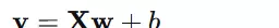
在矩阵形式下，该公式可写作：

损失函数与优化

线性回归的主要目标是确定一组权重 $\mathbf{w}$ 和偏置 $b$，使预测值与实际值之间的差距尽可能小。最常用的损失函数是均方误差（MSE），定义如下：

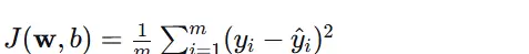
其中 $m$ 代表样本总数，$y_i$ 是实际值，而 $\hat{y}_i$ 则是预测值。

以下代码进一步阐述了线性模型的实现：

import numpy as np
import matplotlib.pyplot as plt
from sklearn.linear_model import LinearRegression, Ridge, Lasso
from sklearn.preprocessing import PolynomialFeatures, StandardScaler
from sklearn.pipeline import Pipeline
from sklearn.metrics import mean_squared_error

# 生成示例数据
np.random.seed(42)
X = np.linspace(0, 10, 100).reshape(-1, 1)
y = 2 * X.squeeze() + 1 + np.random.normal(0, 2, 100)  # y = 2x + 1 + 噪声

# 可视化原始数据
plt.figure(figsize=(10, 6))
plt.scatter(X, y, alpha=0.6, label='数据点')
plt.xlabel('X')
plt.ylabel('y')
plt.title('线性回归示例数据')
plt.legend()
plt.show()

# 训练线性回归模型
model = LinearRegression()
model.fit(X, y)

# 预测
X_test = np.linspace(0, 10, 100).reshape(-1, 1)
y_pred = model.predict(X_test)

# 可视化结果
plt.figure(figsize=(10, 6))
plt.scatter(X, y, alpha=0.6, label='数据点')
plt.plot(X_test, y_pred, 'r-', linewidth=2, label=f'拟合直线: y = {model.coef_[0]:.2f}x + {model.intercept_:.2f}')
plt.xlabel('X')
plt.ylabel('y')
plt.title('线性回归拟合结果')
plt.legend()
plt.show()

print(f"模型系数: {model.coef_[0]:.4f}")
print(f"模型截距: {model.intercept_:.4f}")
print(f"R? 分数: {model.score(X, y):.4f}")

# 多变量线性回归示例
print("\n" + "="*50)
print("多变量线性回归示例")
print("="*50)

# 生成多变量数据
np.random.seed(42)
n_samples = 200

# 生成三个特征
X1 = np.random.normal(0, 1, n_samples)
X2 = np.random.normal(0, 1, n_samples)
X3 = np.random.normal(0, 1, n_samples)

# 生成目标变量：y = 2*X1 + 3*X2 - 1.5*X3 + 噪声
y_multi = 2 * X1 + 3 * X2 - 1.5 * X3 + np.random.normal(0, 0.5, n_samples)

# 组合特征
X_multi = np.column_stack([X1, X2, X3])

# 训练多变量线性回归模型
model_multi = LinearRegression()
model_multi.fit(X_multi, y_multi)

# 输出结果
print("多变量线性回归结果:")
print(f"系数: {model_multi.coef_}")
print(f"截距: {model_multi.intercept_:.4f}")
print(f"R? 分数: {model_multi.score(X_multi, y_multi):.4f}")

# 预测新样本
new_sample = np.array([[1.0, -0.5, 0.3]])
prediction = model_multi.predict(new_sample)
print(f"\n新样本预测: {prediction[0]:.4f}")

# 正则化线性模型比较
print("\n" + "="*50)
print("正则化线性模型比较")
print("="*50)

# 添加一些噪声特征
X_with_noise = np.column_stack([X1, X2, X3, 
                               np.random.normal(0, 1, n_samples),
                               np.random.normal(0, 1, n_samples)])

# 标准化特征
scaler = StandardScaler()
X_scaled = scaler.fit_transform(X_with_noise)

# 划分训练集和测试集
from sklearn.model_selection import train_test_split
X_train, X_test, y_train, y_test = train_test_split(X_scaled, y_multi, test_size=0.3, random_state=42)

# 训练不同模型
models = {
    '线性回归': LinearRegression(),
    'Ridge (L2正则化)': Ridge(alpha=1.0),
    'Lasso (L1正则化)': Lasso(alpha=0.1)
}

results = {}
for name, model in models.items():
    model.fit(X_train, y_train)
    y_pred = model.predict(X_test)
    mse = mean_squared_error(y_test, y_pred)
    results[name] = {
        'model': model,
        'mse': mse,
        'coefficients': model.coef_ if hasattr(model, 'coef_') else None
    }
    print(f"{name} - MSE: {mse:.4f}")

# 比较系数
print("\n系数比较:")
for name, result in results.items():
    if result['coefficients'] is not None:
        print(f"{name}: {np.round(result['coefficients'], 4)}")

1.2.1 分段线性曲线

在现实世界的问题中，许多关系并非简单的线性，而是表现出分段线性的特点。分段线性模型通过将输入空间细分为多个区域，并在每个区域内应用不同的线性函数，从而更好地近似复杂的非线性关系。

分段线性回归原理

分段线性回归的核心思想是将数据分割成若干区间，然后在每个区间内独立拟合线性模型。常见的分段线性模型包括：
- 连续分段线性：确保在断点处连续
- 不连续分段线性：允许在断点处出现跳跃

以下是通过代码实现分段线性回归的方法：

import numpy as np
import matplotlib.pyplot as plt
from sklearn.tree import DecisionTreeRegressor
from sklearn.linear_model import LinearRegression
from sklearn.metrics import mean_squared_error

# 生成分段线性数据
np.random.seed(42)
n_samples = 300
X = np.random.uniform(0, 10, n_samples)

# 定义分段线性函数
def piecewise_linear(x):
    conditions = [x < 3, (x >= 3) & (x < 7), x >= 7]
    functions = [lambda x: 2*x + 1, 
                lambda x: -x + 10, 
                lambda x: 0.5*x + 2.5]
    
    y = np.piecewise(x, conditions, functions)
    return y

y_true = piecewise_linear(X)
y = y_true + np.random.normal(0, 0.5, n_samples)  # 添加噪声

# 可视化原始数据
plt.figure(figsize=(12, 4))

plt.subplot(1, 3, 1)
plt.scatter(X, y, alpha=0.6, s=20, label='带噪声数据')
x_plot = np.linspace(0, 10, 100)
plt.plot(x_plot, piecewise_linear(x_plot), 'r-', linewidth=2, label='真实函数')
plt.xlabel('X')
plt.ylabel('y')
plt.title('原始数据与真实函数')
plt.legend()

# 方法1：使用决策树进行分段线性回归
plt.subplot(1, 3, 2)
tree_model = DecisionTreeRegressor(max_leaf_nodes=10, random_state=42)
tree_model.fit(X.reshape(-1, 1), y)

X_plot = np.linspace(0, 10, 1000).reshape(-1, 1)
y_tree = tree_model.predict(X_plot)

plt.scatter(X, y, alpha=0.6, s=20)
plt.plot(X_plot, y_tree, 'r-', linewidth=2, label='决策树拟合')
plt.xlabel('X')
plt.ylabel('y')
plt.title('决策树分段线性回归')
plt.legend()

# 方法2：手动分段线性回归
plt.subplot(1, 3, 3)

# 定义断点
breakpoints = [3, 7]
segments = [(0, 3), (3, 7), (7, 10)]

colors = ['red', 'green', 'blue']
for i, (start, end) in enumerate(segments):
    # 选择当前段的数据
    mask = (X >= start) & (X < end)
    X_seg = X[mask].reshape(-1, 1)
    y_seg = y[mask]
    
    if len(X_seg) > 1:  # 确保有足够的数据点
        # 在当前段拟合线性模型
        seg_model = LinearRegression()
        seg_model.fit(X_seg, y_seg)
        
        # 预测并绘制当前段
        X_plot_seg = np.linspace(start, end, 100).reshape(-1, 1)
        y_plot_seg = seg_model.predict(X_plot_seg)
        
        plt.plot(X_plot_seg, y_plot_seg, color=colors[i], linewidth=2, 
                label=f'段 {i+1}: y = {seg_model.coef_[0]:.2f}x + {seg_model.intercept_:.2f}')

plt.scatter(X, y, alpha=0.3, s=20, color='gray')
plt.xlabel('X')
plt.ylabel('y')
plt.title('手动分段线性回归')
plt.legend()

plt.tight_layout()
plt.show()

# 评估不同方法
print("分段线性回归方法比较:")
print("=" * 50)

# 方法1：决策树评估
y_pred_tree = tree_model.predict(X.reshape(-1, 1))
mse_tree = mean_squared_error(y, y_pred_tree)
print(f"决策树方法 - MSE: {mse_tree:.4f}")

# 方法2：手动分段评估
y_pred_manual = np.zeros_like(y)
for i, (start, end) in enumerate(segments):
    mask = (X >= start) & (X < end)
    X_seg = X[mask].reshape(-1, 1)
    
    if len(X_seg) > 0:
        seg_model = LinearRegression()
        seg_model.fit(X_seg, y[mask])
        y_pred_manual[mask] = seg_model.predict(X_seg)

mse_manual = mean_squared_error(y, y_pred_manual)
print(f"手动分段方法 - MSE: {mse_manual:.4f}")

# 方法3：简单线性回归对比
simple_lr = LinearRegression()
simple_lr.fit(X.reshape(-1, 1), y)
y_pred_simple = simple_lr.predict(X.reshape(-1, 1))
mse_simple = mean_squared_error(y, y_pred_simple)
print(f"简单线性回归 - MSE: {mse_simple:.4f}")
print(f"简单线性回归方程: y = {simple_lr.coef_[0]:.2f}x + {simple_lr.intercept_:.2f}")

# 复杂分段线性回归示例
print("\n" + "="*50)
print("复杂分段线性回归示例")
print("="*50)

# 生成更复杂的分段线性数据
np.random.seed(123)
X_complex = np.random.uniform(-5, 5, 500)

def complex_piecewise(x):
    conditions = [x < -2, (x >= -2) & (x < 1), (x >= 1) & (x < 3), x >= 3]
    functions = [lambda x: x**2 / 2,  # 抛物线部分
                lambda x: 2*x + 3,   # 线性部分
                lambda x: -x**2 + 4*x + 2,  # 抛物线部分
                lambda x: 0.5*x + 8] # 线性部分
    
    y = np.piecewise(x, conditions, functions)
    return y

y_complex_true = complex_piecewise(X_complex)
y_complex = y_complex_true + np.random.normal(0, 0.3, len(X_complex))

# 使用多个线性段逼近复杂函数
n_segments = 8
breakpoints_complex = np.linspace(-5, 5, n_segments + 1)

plt.figure(figsize=(12, 5))

# 绘制真实函数
x_plot_complex = np.linspace(-5, 5, 1000)
y_plot_true = complex_piecewise(x_plot_complex)

plt.plot(x_plot_complex, y_plot_true, 'b-', linewidth=2, alpha=0.7, label='真实函数')

# 分段拟合
for i in range(n_segments):
    start, end = breakpoints_complex[i], breakpoints_complex[i+1]
    mask = (X_complex >= start) & (X_complex < end)
    X_seg = X_complex[mask].reshape(-1, 1)
    y_seg = y_complex[mask]
    
    if len(X_seg) > 1:
        seg_model = LinearRegression()
        seg_model.fit(X_seg, y_seg)
        
        # 绘制当前段
        X_plot_seg = np.linspace(start, end, 50).reshape(-1, 1)
        y_plot_seg = seg_model.predict(X_plot_seg)
        
        plt.plot(X_plot_seg, y_plot_seg, 'r-', linewidth=2, alpha=0.8)

plt.scatter(X_complex, y_complex, alpha=0.4, s=10, color='gray', label='数据点')
plt.xlabel('X')
plt.ylabel('y')
plt.title('复杂函数的分段线性逼近')
plt.legend()
plt.show()

# 评估逼近效果
y_pred_complex = np.zeros_like(X_complex)
for i in range(n_segments):
    start, end = breakpoints_complex[i], breakpoints_complex[i+1]
    mask = (X_complex >= start) & (X_complex < end)
    X_seg = X_complex[mask].reshape(-1, 1)
    
    if len(X_seg) > 0:
        seg_model = LinearRegression()
        seg_model.fit(X_seg, y_complex[mask])
        y_pred_complex[mask] = seg_model.predict(X_seg)

mse_complex = mean_squared_error(y_complex, y_pred_complex)
print(f"复杂函数分段逼近 - MSE: {mse_complex:.4f}")
print(f"使用 {n_segments} 个线性段")

# 不同分段数量的效果比较
segment_counts = [2, 4, 8, 16, 32]
mse_scores = []

for n_seg in segment_counts:
    breakpoints_temp = np.linspace(-5, 5, n_seg + 1)
    y_pred_temp = np.zeros_like(X_complex)
    
    for i in range(n_seg):
        start, end = breakpoints_temp[i], breakpoints_temp[i+1]
        mask = (X_complex >= start) & (X_complex < end)
        X_seg = X_complex[mask].reshape(-1, 1)
        
        if len(X_seg) > 1:
            seg_model = LinearRegression()
            seg_model.fit(X_seg, y_complex[mask])
            y_pred_temp[mask] = seg_model.predict(X_seg)
    
    mse_temp = mean_squared_error(y_complex, y_pred_temp)
    mse_scores.append(mse_temp)

plt.figure(figsize=(10, 5))
plt.plot(segment_counts, mse_scores, 'bo-', linewidth=2, markersize=8)
plt.xlabel('分段数量')
plt.ylabel('均方误差 (MSE)')
plt.title('分段数量对拟合效果的影响')
plt.grid(True, alpha=0.3)
plt.show()

print("\n分段数量与MSE关系:")
for n_seg, mse_val in zip(segment_counts, mse_scores):
    print(f"{n_seg} 段: MSE = {mse_val:.4f}")

1.2.2 模型变形

在实际的机器学习项目中，为了适应不同的数据特性和问题需求，我们通常需要对基础线性模型进行变形和扩展。这种变形是增强模型表达力的关键。

常见的模型变形技术包括：

• 多项式回归：通过增加特征的高阶项来捕捉非线性关系
• 交互项：考虑不同特征间的相互作用
• 正则化：避免过拟合，提升模型的泛化能力
• 特征变换：例如对数变换、指数变换等

下面是通过代码展示上述模型变形技术的实例：

import numpy as np
import matplotlib.pyplot as plt
from sklearn.preprocessing import PolynomialFeatures
from sklearn.linear_model import LinearRegression, Ridge, Lasso
from sklearn.pipeline import Pipeline
from sklearn.metrics import mean_squared_error, r2_score
from sklearn.model_selection import train_test_split

# 生成非线性数据
np.random.seed(42)
n_samples = 200
X = np.random.uniform(-3, 3, n_samples)
y = 0.5 * X**3 - 2 * X**2 + 1.5 * X + 2 + np.random.normal(0, 1, n_samples)

# 划分训练集和测试集
X_train, X_test, y_train, y_test = train_test_split(X.reshape(-1, 1), y, test_size=0.3, random_state=42)

# 创建不同的多项式模型
degrees = [1, 2, 3, 5, 10]
models = {}

plt.figure(figsize=(15, 10))

for i, degree in enumerate(degrees):
    # 创建多项式回归管道
    polynomial_model = Pipeline([
        ('poly', PolynomialFeatures(degree=degree)),
        ('linear', LinearRegression())
    ])
    
    # 训练模型
    polynomial_model.fit(X_train, y_train)
    
    # 预测
    X_plot = np.linspace(-3, 3, 100).reshape(-1, 1)
    y_plot = polynomial_model.predict(X_plot)
    
    # 计算性能
    y_pred_train = polynomial_model.predict(X_train)
    y_pred_test = polynomial_model.predict(X_test)
    
    train_mse = mean_squared_error(y_train, y_pred_train)
    test_mse = mean_squared_error(y_test, y_pred_test)
    
    models[degree] = {
        'model': polynomial_model,
        'train_mse': train_mse,
        'test_mse': test_mse,
        'predictions': y_plot
    }
    
    # 绘制子图
    plt.subplot(2, 3, i+1)
    plt.scatter(X_train, y_train, alpha=0.6, s=30, label='训练数据')
    plt.scatter(X_test, y_test, alpha=0.6, s=30, label='测试数据', color='red')
    plt.plot(X_plot, y_plot, 'g-', linewidth=2, label=f'多项式拟合 (度={degree})')
    plt.xlabel('X')
    plt.ylabel('y')
    plt.title(f'多项式回归 (度={degree})\n训练MSE: {train_mse:.2f}, 测试MSE: {test_mse:.2f}')
    plt.legend()
    plt.grid(True, alpha=0.3)

plt.tight_layout()
plt.show()

# 比较不同多项式次数的效果
print("多项式回归比较:")
print("=" * 60)
for degree in degrees:
    model_info = models[degree]
    print(f"度 {degree}: 训练MSE = {model_info['train_mse']:.4f}, 测试MSE = {model_info['test_mse']:.4f}")

# 正则化模型比较
print("\n" + "="*60)
print("正则化模型比较")
print("="*60)

# 使用较高次数的多项式（容易过拟合）
degree_high = 15

# 创建不同的正则化模型
regularized_models = {
    '无正则化': Pipeline([
        ('poly', PolynomialFeatures(degree=degree_high)),
        ('linear', LinearRegression())
    ]),
    'Ridge (L2)': Pipeline([
        ('poly', PolynomialFeatures(degree=degree_high)),
        ('linear', Ridge(alpha=1.0))
    ]),
    'Lasso (L1)': Pipeline([
        ('poly', PolynomialFeatures(degree=degree_high)),
        ('linear', Lasso(alpha=0.1, max_iter=10000))
    ])
}

plt.figure(figsize=(15, 5))

for i, (name, model) in enumerate(regularized_models.items()):
    # 训练模型
    model.fit(X_train, y_train)
    
    # 预测
    X_plot = np.linspace(-3, 3, 100).reshape(-1, 1)
    y_plot = model.predict(X_plot)
    
    # 计算性能
    y_pred_train = model.predict(X_train)
    y_pred_test = model.predict(X_test)
    
    train_mse = mean_squared_error(y_train, y_pred_train)
    test_mse = mean_squared_error(y_test, y_pred_test)
    
    # 绘制
    plt.subplot(1, 3, i+1)
    plt.scatter(X_train, y_train, alpha=0.6, s=30, label='训练数据')
    plt.scatter(X_test, y_test, alpha=0.6, s=30, label='测试数据', color='red')
    plt.plot(X_plot, y_plot, 'g-', linewidth=2, label=name)
    plt.xlabel('X')
    plt.ylabel('y')
    plt.title(f'{name}\n训练MSE: {train_mse:.2f}, 测试MSE: {test_mse:.2f}')
    plt.legend()
    plt.grid(True, alpha=0.3)

plt.tight_layout()
plt.show()

# 特征交互项示例
print("\n" + "="*60)
print("特征交互项示例")
print("="*60)

# 生成多特征数据
np.random.seed(42)
n_samples = 300

# 两个特征
X1 = np.random.normal(0, 1, n_samples)
X2 = np.random.normal(0, 1, n_samples)

# 目标变量包含交互效应：y = 2*X1 + 3*X2 + 1.5*X1*X2 + 噪声
y_interaction = 2 * X1 + 3 * X2 + 1.5 * X1 * X2 + np.random.normal(0, 0.5, n_samples)

# 组合特征
X_multi = np.column_stack([X1, X2])

# 划分训练测试集
X_train_multi, X_test_multi, y_train_multi, y_test_multi = train_test_split(
    X_multi, y_interaction, test_size=0.3, random_state=42)

# 不同特征集的模型比较
feature_sets = {
    '仅主效应': PolynomialFeatures(degree=1, include_bias=False),  # 只有X1, X2
    '含交互项': PolynomialFeatures(degree=2, include_bias=False, interaction_only=True),  # X1, X2, X1*X2
    '完整二次项': PolynomialFeatures(degree=2, include_bias=False)  # X1, X2, X1?, X2?, X1*X2
}

results = {}

plt.figure(figsize=(15, 5))

for i, (name, poly_transformer) in enumerate(feature_sets.items()):
    # 创建模型管道
    model_pipeline = Pipeline([
        ('poly', poly_transformer),
        ('linear', LinearRegression())
    ])
    
    # 训练模型
    model_pipeline.fit(X_train_multi, y_train_multi)
    
    # 预测
    y_pred_train = model_pipeline.predict(X_train_multi)
    y_pred_test = model_pipeline.predict(X_test_multi)
    
    # 计算性能
    train_mse = mean_squared_error(y_train_multi, y_pred_train)
    test_mse = mean_squared_error(y_test_multi, y_pred_test)
    train_r2 = r2_score(y_train_multi, y_pred_train)
    test_r2 = r2_score(y_test_multi, y_pred_test)
    
    results[name] = {
        'train_mse': train_mse,
        'test_mse': test_mse,
        'train_r2': train_r2,
        'test_r2': test_r2,
        'model': model_pipeline
    }
    
    # 绘制预测vs实际图
    plt.subplot(1, 3, i+1)
    plt.scatter(y_test_multi, y_pred_test, alpha=0.6)
    plt.plot([y_test_multi.min(), y_test_multi.max()], 
             [y_test_multi.min(), y_test_multi.max()], 'r--', linewidth=2)
    plt.xlabel('实际值')
    plt.ylabel('预测值')
    plt.title(f'{name}\n测试R?: {test_r2:.4f}')
    plt.grid(True, alpha=0.3)

plt.tight_layout()
plt.show()

# 输出结果比较
print("\n特征交互效应模型比较:")
print("=" * 70)
for name, result in results.items():
    print(f"{name:15} | 训练MSE: {result['train_mse']:.4f} | 测试MSE: {result['test_mse']:.4f} | "
          f"训练R?: {result['train_r2']:.4f} | 测试R?: {result['test_r2']:.4f}")

# 特征变换示例
print("\n" + "="*60)
print("特征变换示例")
print("="*60)

# 生成指数关系数据
np.random.seed(42)
X_exp = np.random.uniform(1, 10, 200)
y_exp = 2 * np.exp(0.5 * X_exp) + np.random.normal(0, 10, 200)

# 不同的特征变换
transformations = {
    '原始特征': lambda x: x.reshape(-1, 1),
    '对数变换': lambda x: np.log(x).reshape(-1, 1),
    '平方根变换': lambda x: np.sqrt(x).reshape(-1, 1),
    '平方变换': lambda x: (x**2).reshape(-1, 1)
}

plt.figure(figsize=(15, 10))

for i, (name, transform_func) in enumerate(transformations.items()):
    # 应用特征变换
    X_transformed = transform_func(X_exp)
    
    # 训练线性模型
    model = LinearRegression()
    model.fit(X_transformed, y_exp)
    
    # 预测
    X_plot = np.linspace(1, 10, 100)
    X_plot_transformed = transform_func(X_plot)
    y_plot = model.predict(X_plot_transformed)
    
    # 计算性能
    y_pred = model.predict(X_transformed)
    r2 = r2_score(y_exp, y_pred)
    
    # 绘制
    plt.subplot(2, 2, i+1)
    plt.scatter(X_exp, y_exp, alpha=0.6, s=30, label='数据点')
    plt.plot(X_plot, y_plot, 'r-', linewidth=2, label=f'拟合曲线 (R?={r2:.4f})')
    plt.xlabel('X' if name == '原始特征' else f'变换后的X ({name})')
    plt.ylabel('y')
    plt.title(f'{name} - 线性回归拟合')
    plt.legend()
    plt.grid(True, alpha=0.3)

plt.tight_layout()
plt.show()

# 输出变换效果
print("\n特征变换效果比较:")
print("=" * 50)
for name, transform_func in transformations.items():
    X_transformed = transform_func(X_exp)
    model = LinearRegression()
    model.fit(X_transformed, y_exp)
    y_pred = model.predict(X_transformed)
    r2 = r2_score(y_exp, y_pred)
    print(f"{name:12}: R? = {r2:.4f}")

1.2.3 机器学习框架

机器学习框架提供了实现各类机器学习算法的标准工具和接口。掌握这些框架的基本原理和使用技巧对于实际开发至关重要。

主流的机器学习框架有：

• Scikit-learn：适用于传统机器学习算法的库
• TensorFlow/Keras：专为深度学习和神经网络设计
• PyTorch：面向研究的深度学习框架
• XGBoost/LightGBM：专注于梯度提升树模型

以下是利用这些框架进行基本操作的代码示例：

import numpy as np
import matplotlib.pyplot as plt
from sklearn import datasets
from sklearn.model_selection import train_test_split, cross_val_score, GridSearchCV
from sklearn.preprocessing import StandardScaler
from sklearn.ensemble import RandomForestClassifier, GradientBoostingClassifier
from sklearn.svm import SVC
from sklearn.metrics import classification_report, confusion_matrix, accuracy_score
import tensorflow as tf
from tensorflow import keras
import xgboost as xgb
import warnings
warnings.filterwarnings('ignore')

# 加载鸢尾花数据集
iris = datasets.load_iris()
X, y = iris.data, iris.target

print("数据集信息:")
print(f"特征形状: {X.shape}")
print(f"目标形状: {y.shape}")
print(f"特征名称: {iris.feature_names}")
print(f"目标类别: {iris.target_names}")
print(f"类别分布: {np.bincount(y)}")

# 数据预处理
scaler = StandardScaler()
X_scaled = scaler.fit_transform(X)

# 划分数据集
X_train, X_test, y_train, y_test = train_test_split(X_scaled, y, test_size=0.3, 
                                                    random_state=42, stratify=y)

print(f"\n训练集大小: {X_train.shape[0]}")
print(f"测试集大小: {X_test.shape[0]}")

# 定义多个模型进行比较
models = {
    '随机森林': RandomForestClassifier(n_estimators=100, random_state=42),
    '梯度提升': GradientBoostingClassifier(n_estimators=100, random_state=42),
    '支持向量机': SVC(kernel='rbf', random_state=42),
    'XGBoost': xgb.XGBClassifier(n_estimators=100, random_state=42)
}

# 训练和评估模型
results = {}

plt.figure(figsize=(15, 10))

for i, (name, model) in enumerate(models.items()):
    # 训练模型
    model.fit(X_train, y_train)
    
    # 预测
    y_pred = model.predict(X_test)
    
    # 计算准确率
    accuracy = accuracy_score(y_test, y_pred)
    
    # 交叉验证
    cv_scores = cross_val_score(model, X_scaled, y, cv=5)
    
    results[name] = {
        'model': model,
        'accuracy': accuracy,
        'cv_mean': cv_scores.mean(),
        'cv_std': cv_scores.std(),
        'predictions': y_pred
    }
    
    # 绘制混淆矩阵
    plt.subplot(2, 2, i+1)
    cm = confusion_matrix(y_test, y_pred)
    plt.imshow(cm, interpolation='nearest', cmap=plt.cm.Blues)
    plt.title(f'{name}\n准确率: {accuracy:.3f}')
    plt.colorbar()
    tick_marks = np.arange(len(iris.target_names))
    plt.xticks(tick_marks, iris.target_names, rotation=45)
    plt.yticks(tick_marks, iris.target_names)
    plt.xlabel('预测标签')
    plt.ylabel('真实标签')
    
    # 在图中添加数值
    thresh = cm.max() / 2.
    for i_arr, j_arr in np.ndindex(cm.shape):
        plt.text(j_arr, i_arr, format(cm[i_arr, j_arr], 'd'),
                horizontalalignment="center",
                color="white" if cm[i_arr, j_arr] > thresh else "black")

plt.tight_layout()
plt.show()

# 输出详细结果
print("模型性能比较:")
print("=" * 80)
for name, result in results.items():
    print(f"{name:12} | 测试准确率: {result['accuracy']:.4f} | "
          f"交叉验证: {result['cv_mean']:.4f} ± {result['cv_std']:.4f}")

# 超参数调优示例
print("\n" + "="*60)
print("超参数调优示例 (随机森林)")
print("="*60)

# 定义参数网格
param_grid = {
    'n_estimators': [50, 100, 200],
    'max_depth': [3, 5, 7, None],
    'min_samples_split': [2, 5, 10]
}

# 网格搜索
grid_search = GridSearchCV(
    RandomForestClassifier(random_state=42),
    param_grid,
    cv=5,
    scoring='accuracy',
    n_jobs=-1
)

grid_search.fit(X_train, y_train)

print(f"最佳参数: {grid_search.best_params_}")
print(f"最佳交叉验证分数: {grid_search.best_score_:.4f}")
print(f"测试集准确率: {grid_search.score(X_test, y_test):.4f}")

# 特征重要性可视化
best_rf = grid_search.best_estimator_
importances = best_rf.feature_importances_
indices = np.argsort(importances)[::-1]

plt.figure(figsize=(10, 6))
plt.title("随机森林特征重要性")
plt.bar(range(X.shape[1]), importances[indices])
plt.xticks(range(X.shape[1]), [iris.feature_names[i] for i in indices], rotation=45)
plt.tight_layout()
plt.show()

# 使用TensorFlow/Keras构建神经网络
print("\n" + "="*60)
print("TensorFlow/Keras 神经网络示例")
print("="*60)

# 构建简单的神经网络模型
keras_model = keras.Sequential([
    keras.layers.Dense(64, activation='relu', input_shape=(X_train.shape[1],)),
    keras.layers.Dropout(0.3),
    keras.layers.Dense(32, activation='relu'),
    keras.layers.Dropout(0.3),
    keras.layers.Dense(3, activation='softmax')  # 3个输出类别
])

# 编译模型
keras_model.compile(
    optimizer='adam',
    loss='sparse_categorical_crossentropy',
    metrics=['accuracy']
)

print("神经网络结构:")
keras_model.summary()

# 训练模型
history = keras_model.fit(
    X_train, y_train,
    epochs=100,
    batch_size=16,
    validation_split=0.2,
    verbose=0
)

# 评估模型
test_loss, test_accuracy = keras_model.evaluate(X_test, y_test, verbose=0)
print(f"\n神经网络测试准确率: {test_accuracy:.4f}")

# 绘制训练历史
plt.figure(figsize=(12, 4))

plt.subplot(1, 2, 1)
plt.plot(history.history['accuracy'], label='训练准确率')
plt.plot(history.history['val_accuracy'], label='验证准确率')
plt.xlabel('Epoch')
plt.ylabel('准确率')
plt.title('训练和验证准确率')
plt.legend()

plt.subplot(1, 2, 2)
plt.plot(history.history['loss'], label='训练损失')
plt.plot(history.history['val_loss'], label='验证损失')
plt.xlabel('Epoch')
plt.ylabel('损失')
plt.title('训练和验证损失')
plt.legend()

plt.tight_layout()
plt.show()

# 模型集成示例
print("\n" + "="*60)
print("模型集成示例")
print("="*60)

from sklearn.ensemble import VotingClassifier

# 创建集成模型
voting_clf = VotingClassifier(
    estimators=[
        ('rf', RandomForestClassifier(n_estimators=100, random_state=42)),
        ('gb', GradientBoostingClassifier(n_estimators=100, random_state=42)),
        ('svc', SVC(kernel='rbf', probability=True, random_state=42))
    ],
    voting='soft'  # 使用软投票（概率平均）
)

# 训练集成模型
voting_clf.fit(X_train, y_train)

# 评估集成模型
voting_accuracy = voting_clf.score(X_test, y_test)
print(f"集成模型准确率: {voting_accuracy:.4f}")

# 比较所有模型
all_models = dict(models)
all_models['神经网络'] = {'accuracy': test_accuracy}
all_models['集成模型'] = {'accuracy': voting_accuracy}
all_models['调优随机森林'] = {'accuracy': grid_search.score(X_test, y_test)}

# 绘制准确率比较图
model_names = list(all_models.keys())
accuracies = [all_models[name]['accuracy'] if isinstance(all_models[name], dict) 
             else all_models[name].score(X_test, y_test) for name in model_names]

plt.figure(figsize=(12, 6))
bars = plt.bar(model_names, accuracies, color=['skyblue', 'lightgreen', 'lightcoral', 
                                              'gold', 'violet', 'orange'])
plt.ylabel('准确率')
plt.title('不同机器学习模型准确率比较')
plt.ylim(0.8, 1.0)
plt.xticks(rotation=45)

# 在柱子上添加数值
for bar, accuracy in zip(bars, accuracies):
    plt.text(bar.get_x() + bar.get_width()/2, bar.get_height() + 0.005,
            f'{accuracy:.4f}', ha='center', va='bottom')

plt.tight_layout()
plt.show()

print("\n最终模型比较:")
print("=" * 50)
for name, accuracy in zip(model_names, accuracies):
    print(f"{name:20}: {accuracy:.4f}")

# 模型部署准备示例
print("\n" + "="*60)
print("模型部署准备示例")
print("="*60)

# 保存最佳模型
import joblib

# 保存模型和缩放器
joblib.dump(best_rf, 'best_random_forest_model.pkl')
joblib.dump(scaler, 'scaler.pkl')

print("模型和预处理对象已保存")

# 加载模型并进行预测的示例
def predict_new_sample(model_path, scaler_path, new_data):
    """
    加载保存的模型并对新样本进行预测
    """
    # 加载模型和缩放器
    loaded_model = joblib.load(model_path)
    loaded_scaler = joblib.load(scaler_path)
    
    # 预处理新数据
    new_data_scaled = loaded_scaler.transform(new_data)
    
    # 进行预测
    predictions = loaded_model.predict(new_data_scaled)
    probabilities = loaded_model.predict_proba(new_data_scaled)
    
    return predictions, probabilities

# 测试新样本预测
new_samples = np.array([
    [5.1, 3.5, 1.4, 0.2],  # 应该是setosa
    [6.7, 3.0, 5.2, 2.3],  # 应该是virginica
    [5.9, 2.8, 4.3, 1.3]   # 应该是versicolor
])

predictions, probabilities = predict_new_sample('best_random_forest_model.pkl', 'scaler.pkl', new_samples)

print("\n新样本预测结果:")
for i, (pred, prob) in enumerate(zip(predictions, probabilities)):
    print(f"样本 {i+1}: 预测类别 = {iris.target_names[pred]}, "
          f"概率 = {np.max(prob):.4f} ({iris.target_names[pred]})")

本章节通过具体案例和详尽的Python代码，全面介绍了机器学习的基础知识。从简单的线性模型到复杂的分段线性回归，再到模型变形技术和机器学习框架的应用，我们详细探讨了机器学习解决实际问题的全流程。

关键要点总结：

• 案例学习：从问题定义到模型应用的全过程展示
• 线性模型：作为机器学习的基础，理解其原理非常关键
• 分段线性曲线：能够处理复杂的非线性关系
• 模型变形：技术可以大幅提高模型的表达能力
• 机器学习框架：提供了标准化的工具和最佳实践

这些基础知识和技术为后续学习更复杂的机器学习算法和深度学习模型奠定了坚实的基础。

扫码加我 拉你入群

请注明：姓名-公司-职位

以便审核进群资格，未注明则拒绝

分享0 收藏0 回帖

关键词：机器学习 第1章 randomForest coefficients scikit-learn