请选择 进入手机版 | 继续访问电脑版
楼主: oliyiyi
1887 2

A Quick Introduction to Neural Networks [推广有奖]

版主

泰斗

0%

还不是VIP/贵宾

-

TA的文库  其他...

计量文库

威望
7
论坛币
272091 个
通用积分
31269.1753
学术水平
1435 点
热心指数
1554 点
信用等级
1345 点
经验
383778 点
帖子
9599
精华
66
在线时间
5466 小时
注册时间
2007-5-21
最后登录
2024-3-21

初级学术勋章 初级热心勋章 初级信用勋章 中级信用勋章 中级学术勋章 中级热心勋章 高级热心勋章 高级学术勋章 高级信用勋章 特级热心勋章 特级学术勋章 特级信用勋章

oliyiyi 发表于 2016-11-10 15:39:38 |显示全部楼层 |坛友微信交流群

+2 论坛币
k人 参与回答

经管之家送您一份

应届毕业生专属福利!

求职就业群
赵安豆老师微信:zhaoandou666

经管之家联合CDA

送您一个全额奖学金名额~ !

感谢您参与论坛问题回答

经管之家送您两个论坛币!

+2 论坛币

By Ujjwal Karn.

An Artificial Neural Network (ANN) is a computational model that is inspired by the way biological neural networks in the human brain process information. Artificial Neural Networks have generated a lot of excitement in Machine Learning research and industry, thanks to many breakthrough results in speech recognition, computer vision and text processing. In this blog post we will try to develop an understanding of a particular type of Artificial Neural Network called the Multi Layer Perceptron.

A Single Neuron

The basic unit of computation in a neural network is the neuron, often called a node or unit. It receives input from some other nodes, or from an external source and computes an output. Each input has an associated weight (w), which is assigned on the basis of its relative importance to other inputs. The node applies a function f (defined below) to the weighted sum of its inputs as shown in Figure 1 below:

Figure 1: a single neuron

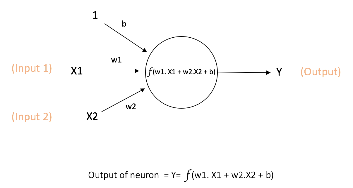
The above network takes numerical inputs X1 and X2 and has weights w1 and w2 associated with those inputs. Additionally, there is another input 1 with weight b (called the Bias) associated with it. We will learn more details about role of the bias later.

The output Y from the neuron is computed as shown in the Figure 1. The function f is non-linear and is called the Activation Function. The purpose of the activation function is to introduce non-linearity into the output of a neuron. This is important because most real world data is non linear and we want neurons to learn thesenon linear representations.

Every activation function (or non-linearity) takes a single number and performs a certain fixed mathematical operation on it [2]. There are several activation functions you may encounter in practice:

  • Sigmoid: takes a real-valued input and squashes it to range between 0 and 1

σ(x) = 1 / (1 + exp(−x))

  • tanh: takes a real-valued input and squashes it to the range [-1, 1]

tanh(x) = 2σ(2x) − 1

  • ReLU: ReLU stands for Rectified Linear Unit. It takes a real-valued input and thresholds it at zero (replaces negative values with zero)

f(x) = max(0, x)

The below figures [2] show each of the above activation functions.

Figure 2: different activation functions

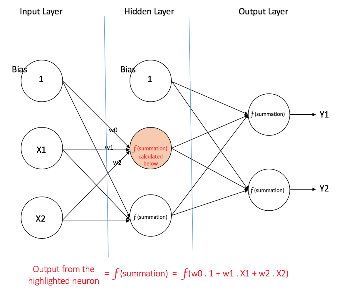
Importance of Bias: The main function of Bias is to provide every node with a trainable constant value (in addition to the normal inputs that the node receives). See this link to learn more about the role of bias in a neuron.
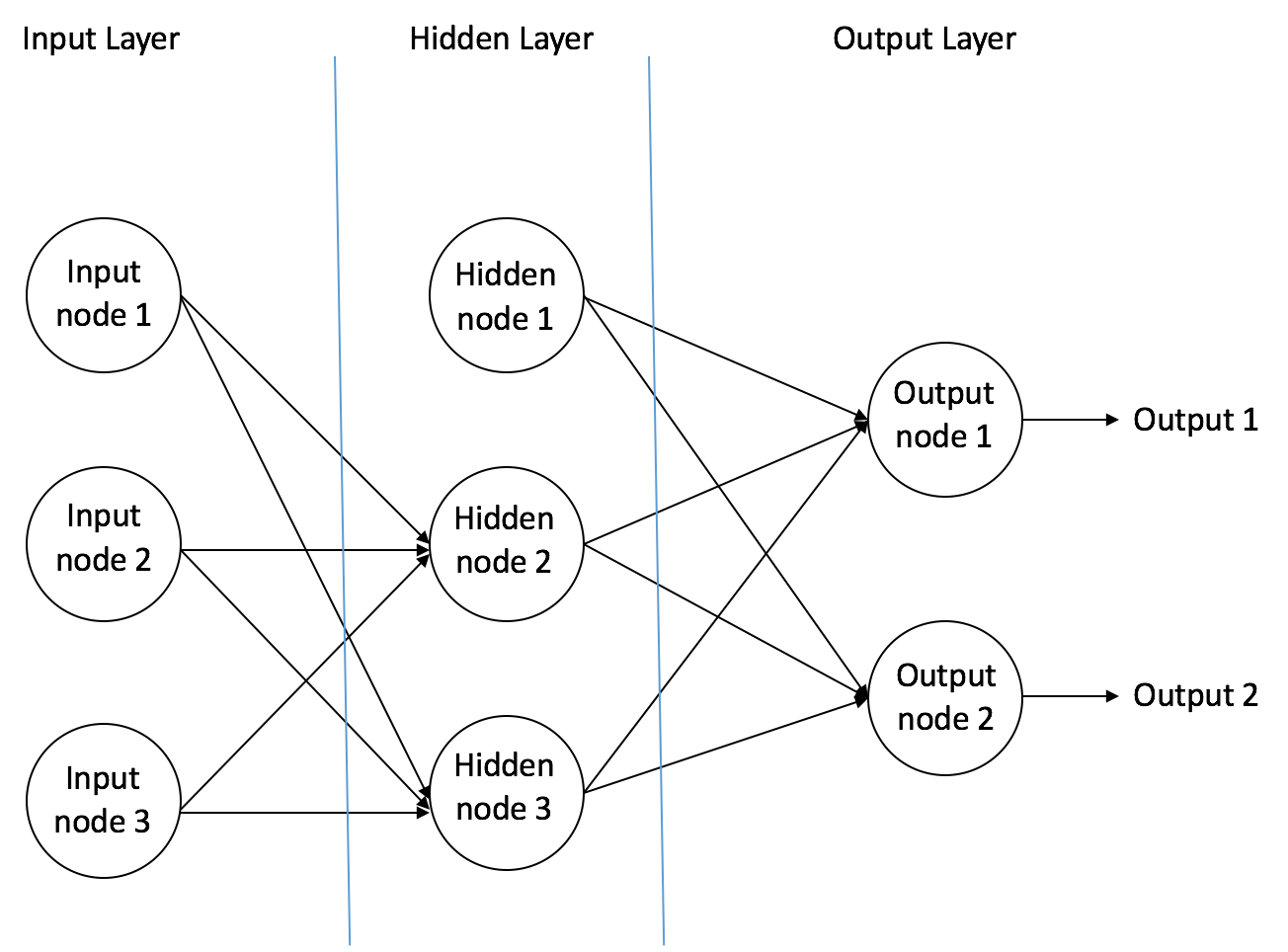
Feedforward Neural Network

The feedforward neural network was the first and simplest type of artificial neural network devised [3]. It contains multiple neurons (nodes) arranged in layers. Nodes from adjacent layers have connections or edges between them. All these connections have weights associated with them.

An example of a feedforward neural network is shown in Figure 3.

Figure 3: an example of feedforward neural network
二维码

扫码加我 拉你入群

请注明:姓名-公司-职位

以便审核进群资格,未注明则拒绝

关键词:introduction troduction Networks network Neural particular generated industry computer research

缺少币币的网友请访问有奖回帖集合
https://bbs.pinggu.org/thread-3990750-1-1.html
oliyiyi 发表于 2016-11-10 15:40:15 |显示全部楼层 |坛友微信交流群

A feedforward neural network can consist of three types of nodes:

  • Input Nodes - The Input nodes provide information from the outside world to the network and are together referred to as the "Input Layer". No computation is performed in any of the Input nodes - they just pass on the information to the hidden nodes.
  • Hidden Nodes - The Hidden nodes have no direct connection with the outside world (hence the name "hidden"). They perform computations and transfer information from the input nodes to the output nodes. A collection of hidden nodes forms a "Hidden Layer". While a feedforward network will only have a single input layer and a single output layer, it can have zero or multiple Hidden Layers.
  • Output Nodes - The Output nodes are collectively referred to as the "Output Layer" and are responsible for computations and transferring information from the network to the outside world.

In a feedforward network, the information moves in only one direction - forward - from the input nodes, through the hidden nodes (if any) and to the output nodes. There are no cycles or loops in the network [3] (this property of feed forward networks is different from Recurrent Neural Networks in which the connections between the nodes form a cycle).

Two examples of feedforward networks are given below:

  • Single Layer Perceptron - This is the simplest feedforward neural network [4] and does not contain any hidden layer. You can learn more about Single Layer Perceptrons in [4], [5], [6], [7].

  • Multi Layer Perceptron - A Multi Layer Perceptron has one or more hidden layers. We will only discuss Multi Layer Perceptrons below since they are more useful than Single Layer Perceptons for practical applications today.


Multi Layer Perceptron

A Multi Layer Perceptron (MLP) contains one or more hidden layers (apart from one input and one output layer). While a single layer perceptron can only learn linear functions, a multi layer perceptron can also learn non - linear functions.

Figure 4 shows a multi layer perceptron with a single hidden layer. Note that all connections have weights associated with them, but only three weights (w0, w1, w2) are shown in the figure.

Input Layer: The Input layer has three nodes. The Bias node has a value of 1. The other two nodes take X1 and X2 as external inputs (which are numerical values depending upon the input dataset). As discussed above, no computation is performed in the Input layer, so the outputs from nodes in the Input layer are 1, X1 and X2 respectively, which are fed into the Hidden Layer.

Hidden Layer: The Hidden layer also has three nodes with the Bias node having an output of 1. The output of the other two nodes in the Hidden layer depends on the outputs from the Input layer (1, X1, X2) as well as the weights associated with the connections (edges). Figure 4 shows the output calculation for one of the hidden nodes (highlighted). Similarly, the output from other hidden node can be calculated. Remember that f refers to the activation function. These outputs are then fed to the nodes in the Output layer.

Figure 4: a multi layer perceptron having one hidden layer

Output Layer: The Output layer has two nodes which take inputs from the Hidden layer and perform similar computations as shown for the highlighted hidden node. The values calculated (Y1 and Y2) as a result of these computations act as outputs of the Multi Layer Perceptron.

Given a set of features X = (x1, x2, ...) and a target y, a Multi Layer Perceptron can learn the relationship between the features and the target, for either classification or regression.

Lets take an example to understand Multi Layer Perceptrons better. Suppose we have the following student-marks dataset:

The two input columns show the number of hours the student has studied and the mid term marks obtained by the student. The Final Result column can have two values 1 or 0 indicating whether the student passed in the final term. For example, we can see that if the student studied 35 hours and had obtained 67 marks in the mid term, he / she ended up passing the final term.

Now, suppose, we want to predict whether a student studying 25 hours and having 70 marks in the mid term will pass the final term.

This is a binary classification problem where a multi layer perceptron can learn from the given examples (training data) and make an informed prediction given a new data point. We will see below how a multi layer perceptron learns such relationships.

Training our MLP: The Back-Propagation Algorithm

The process by which a Multi Layer Perceptron learns is called the Backpropagation algorithm. I would recommend reading this Quora answer by Hemanth Kumar (quoted below) which explains Backpropagation clearly.

Backward Propagation of Errors, often abbreviated as BackProp is one of the several ways in which an artificial neural network (ANN) can be trained. It is a supervised training scheme, which means, it learns from labeled training data (there is a supervisor, to guide its learning).

To put in simple terms, BackProp is like "learning from mistakes". The supervisor corrects the ANN whenever it makes mistakes.

An ANN consists of nodes in different layers; input layer, intermediate hidden layer(s) and the output layer. The connections between nodes of adjacent layers have "weights" associated with them. The goal of learning is to assign correct weights for these edges. Given an input vector, these weights determine what the output vector is.

In supervised learning, the training set is labeled. This means, for some given inputs, we know the desired/expected output (label).

BackProp Algorithm:
Initially all the edge weights are randomly assigned. For every input in the training dataset, the ANN is activated and its output is observed. This output is compared with the desired output that we already know, and the error is "propagated" back to the previous layer. This error is noted and the weights are "adjusted" accordingly. This process is repeated until the output error is below a predetermined threshold.

Once the above algorithm terminates, we have a "learned" ANN which, we consider is ready to work with "new" inputs. This ANN is said to have learned from several examples (labeled data) and from its mistakes (error propagation).

Now that we have an idea of how Backpropagation works, lets come back to our student-marks dataset shown above.


缺少币币的网友请访问有奖回帖集合
https://bbs.pinggu.org/thread-3990750-1-1.html

使用道具

oliyiyi 发表于 2016-11-10 15:41:24 |显示全部楼层 |坛友微信交流群

The Multi Layer Perceptron shown in Figure 5 (adapted from Sebastian Raschka's excellent visual explanation of the backpropagation algorithm) has two nodes in the input layer (apart from the Bias node) which take the inputs 'Hours Studied' and 'Mid Term Marks'. It also has a hidden layer with two nodes (apart from the Bias node). The output layer has two nodes as well - the upper node outputs the probability of 'Pass' while the lower node outputs the probability of 'Fail'.

In classification tasks, we generally use a Softmax function as the Activation Function in the Output layer of the Multi Layer Perceptron to ensure that the outputs are probabilities and they add up to 1. The Softmax function takes a vector of arbitrary real-valued scores and squashes it to a vector of values between zero and one that sum to one. So, in this case,

Probability (Pass) + Probability (Fail) = 1

Step 1: Forward Propagation

All weights in the network are randomly assigned. Lets consider the hidden layer node marked V in Figure 5 below. Assume the weights of the connections from the inputs to that node are w1, w2 and w3 (as shown).

The network then takes the first training example as input (we know that for inputs 35 and 67, the probability of Pass is 1).

  • Input to the network = [35, 67]
  • Desired output from the network (target) = [1, 0]

Then output V from the node in consideration can be calculated as below (f is an activation function such as sigmoid):

V = f (1*w1 + 35*w2 + 67*w3)

Similarly, outputs from the other node in the hidden layer is also calculated. The outputs of the two nodes in the hidden layer act as inputs to the two nodes in the output layer. This enables us to calculate output probabilities from the two nodes in output layer.

Suppose the output probabilities from the two nodes in the output layer are 0.4 and 0.6 respectively (since the weights are randomly assigned, outputs will also be random). We can see that the calculated probabilities (0.4 and 0.6) are very far from the desired probabilities (1 and 0 respectively), hence the network in Figure 5 is said to have an 'Incorrect Output'.

Figure 5: forward propagation step in a multi layer perceptron

Step 2: Back Propagation and Weight Updating

We calculate the total error at the output nodes and propagate these errors back through the network using Backpropagation to calculate the gradients. Then we use an optimization method such as Gradient Descent to 'adjust' all weights in the network with an aim of reducing the error at the output layer. This is shown in the Figure 6 below (ignore the mathematical equations in the figure for now).

Suppose that the new weights associated with the node in consideration are w4, w5 and w6 (after Backpropagation and adjusting weights).

Figure 6: backward propagation and weight updation step in a multi layer perceptron

If we now input the same example to the network again, the network should perform better than before since the weights have now been adjusted to minimize the error in prediction. As shown in Figure 7, the errors at the output nodes now reduce to [0.2, -0.2] as compared to [0.6, -0.4] earlier. This means that our network has learned to correctly classify our first training example.

Figure 7: the MLP network now performs better on the same input

We repeat this process with all other training examples in our dataset. Then, our network is said to have learned those examples.

If we now want to predict whether a student studying 25 hours and having 70 marks in the mid term will pass the final term, we go through the forward propagation step and find the output probabilities for Pass and Fail.

I have avoided mathematical equations and explanation of concepts such as 'Gradient Descent' here and have rather tried to develop an intuition for the algorithm. For a more mathematically involved discussion of the Backpropagation algorithm, refer to this link.

3d Visualization of a Multi Layer Perceptron

Adam Harley has created a 3d visualization of a Multi Layer Perceptron which has already been trained (using Backpropagation) on the MNIST Database of handwritten digits.

The network takes 784 numeric pixel values as inputs from a 28 x 28 image of a handwritten digit (it has 784 nodes in the Input Layer corresponding to pixels). The network has 300 nodes in the first hidden layer, 100 nodes in the second hidden layer, and 10 nodes in the output layer (corresponding to the 10 digits) [15].

Although the network described here is much larger (uses more hidden layers and nodes) compared to the one we discussed in the previous section, all computations in the forward propagation step and backpropagation step are done in the same way (at each node) as discussed before.

Figure 8 shows the network when the input is the digit '5'.

Figure 8: visualizing the network for an input of '5'

A node which has a higher output value than others is represented by a brighter color. In the Input layer, the bright nodes are those which receive higher numerical pixel values as input. Notice how in the output layer, the only bright node corresponds to the digit 5 (it has an output probability of 1, which is higher than the other nine nodes which have an output probability of 0). This indicates that the MLP has correctly classified the input digit. I highly recommend playing around with this visualization and observing connections between nodes of different layers.


缺少币币的网友请访问有奖回帖集合
https://bbs.pinggu.org/thread-3990750-1-1.html

使用道具

您需要登录后才可以回帖 登录 | 我要注册

本版微信群
加好友,备注jltj
拉您入交流群

京ICP备16021002-2号 京B2-20170662号 京公网安备 11010802022788号 论坛法律顾问:王进律师 知识产权保护声明   免责及隐私声明

GMT+8, 2024-3-29 23:40