A gentle introduction to decision trees using R

是 否 +2 论坛币

k人 参与回答

经管之家送您一份

应届毕业生专属福利!

求职就业群

赵安豆老师微信：zhaoandou666

经管之家联合CDA

送您一个全额奖学金名额~ !

立即领取

感谢您参与论坛问题回答

经管之家送您两个论坛币！

+2 论坛币

Introduction

Most techniques of predictive analytics have their origins in probability or statistical theory (see my post on Naïve Bayes, for example).  In this post I’ll look at one that has more a commonplace origin: the way in which humans make decisions.  When making decisions, we typically identify the options available and then evaluate them based on criteria that are important to us.  The intuitive appeal of such a procedure is in no small measure due to the fact that it can be easily explained through a visual. Consider the following graphic, for example:

[color=rgb(255, 255, 255) !important]

扫码加我 拉你入群

请注明：姓名-公司-职位

以便审核进群资格，未注明则拒绝

分享0 收藏3 回帖

关键词：introduction troduction Decision Gentle intro techniques available important procedure criteria

(Original image: https://www.flickr.com/photos/dullhunk/7214525854, Credit: Duncan Hull)

The tree structure depicted here provides a neat, easy-to-follow description of the issue under consideration and its resolution. The decision procedure is based on asking a series of questions, each of which serve to further reduce the domain of possibilities. The predictive technique I discuss in this post,classification and regression trees (CART), works in much the same fashion. It was invented by Leo Breiman and his colleagues in the 1970s.

In what follows, I will use the open source software, R. If you are new to R,   you may want to follow this link for more on the basics of setting up and installing it. Note that the R implementation of the CART algorithm is called RPART (Recursive Partitioning And Regression Trees). This is essentially because Breiman and Co. trademarked the term CART. As some others have pointed out, it is somewhat ironical that the algorithm is now commonly referred to as RPART rather than by the term coined by its inventors.

A bit about the algorithm

The rpart algorithm works by splitting the dataset recursively, which means that the subsets that arise from a split are further split until a predetermined termination criterion is reached.  At each step, the split is made based on the independent variable that results in the largest possible reduction in heterogeneityof the dependent (predicted) variable.

Splitting rules can be constructed in many different ways, all of which are based on the notion of impurity-  a measure of the degree of heterogeneity of the leaf nodes. Put another way, a leaf node that contains a single class is homogeneous and has impurity=0.   There are three popular impurity quantification methods: Entropy (aka information gain), Gini Index and Classification Error.  Check out this article for a simple explanation of the three methods.

The rpart algorithm offers the entropy  and Gini index methods as choices. There is a fair amount of fact and opinion on the Web about which method is better. Here are some of the better articles I’ve come across:

https://www.quora.com/Are-gini-index-entropy-or-classification-error-measures-causing-any-difference-on-Decision-Tree-classification

http://stats.stackexchange.com/questions/130155/when-to-use-gini-impurity-and-when-to-use-information-gain

https://www.garysieling.com/blog/sklearn-gini-vs-entropy-criteria

http://www.salford-systems.com/resources/whitepapers/114-do-splitting-rules-really-matter

The answer as to which method is the best is: it depends.  Given this, it may be prudent to try out a couple of methods and pick the one that works best for your problem.

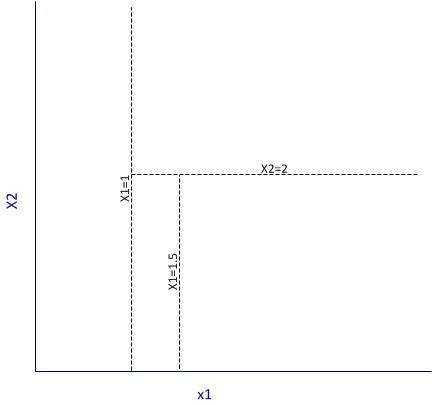
Regardless of the method chosen, the splitting rules partition the decision space (a fancy word for the entire dataset) into rectangular regions each of which correspond to a split. Consider the following simple example with two predictors x1 and x2. The first split is at x1=1 (which splits the decision space into two regions x1<1 and x1>1), the second at x2=2, which splits the (x1>1) region into 2 sub-regions, and finally x1=1.5 which splits the (x1>1,x2>2) sub-region further.

[color=rgb(255, 255, 255) !important]

Figure 2: Example of partitioning

It is important to note that the algorithm works by making the best possible choice at each particular stage, without any consideration of whether those choices remain optimal in future stages. That is, the algorithm makes a locally optimal decision at each stage. It is thus quite possible that such a choice at one stage turns out to be sub-optimal in the overall scheme of things.  In other words,  the algorithm does not find a globally optimal tree.

Another important point relates to well-known bias-variance tradeoff in machine learning, which in simple terms is a tradeoff between the degree to which a model fits the training data and its predictive accuracy.  This refers to the general rule that beyond a point, it is counterproductive to improve the fit of a model to the training data as this increases the likelihood of overfitting.  It is easy to see that deep trees are more likely to overfit the data than shallow ones. One obvious way to control such overfitting is to construct shallower trees by stopping the algorithm at an appropriate point based on whether a split significantly improves the fit.  Another is to grow a tree unrestricted and then prune it back using an appropriate criterion. The rpart algorithm takes the latter approach.

Here is how it works in brief:

Essentially one minimises the cost,  , a quantity that is a  linear combination of the error (essentially, the fraction of misclassified instances, or variance in the case of a continuous variable),   and the number of leaf nodes in the tree, :

First, we note that when , this simply returns the original fully grown tree. As increases, we incur a penalty that is proportional to the number of leaf nodes.  This tends to cause the minimum cost to occur for a tree that is a subtree of the original one (since a subtree will have a smaller number of leaf nodes). In practice we vary and pick the value that gives the subtree that results in the smallest cross-validated prediction error.  One does not have to worry about programming this because the rpart algorithm actually computes the errors for different values of for us. All we need to do is pick the value of the coefficient that gives the lowest cross-validated error. I will illustrate this in detail in the next section.

An implication of their tendency to overfit data is that decision trees tend to be sensitive to relatively minor changes in the training datasets. Indeed, small differences can lead to radically different looking trees. Pruning addresses this to an extent, but does not resolve it completely.  A better resolution is offered by the so-called ensemble methods that average over many differently constructed trees. I’ll discuss one such method at length in a future post.

Finally, I should also mention that decision trees can be used for both classification and regression problems (i.e. those in which the predicted variable is discrete and continuous respectively).  I’ll demonstrate both types of problems in the next two sections.

Classification trees using rpart

To demonstrate classification trees, we’ll use the Ionosphere dataset available in the mlbench package in R. I have chosen this dataset because it nicely illustrates the points I wish to make in this post. In general, you will almost always find that algorithms that work fine on classroom datasets do not work so well in the real world…but of course, you know that already!

We begin by setting the working directory, loading the required packages (rpart and mlbench) and then loading the Ionosphere dataset.

#set working directory if needed (modify path as needed)
setwd(“C:/Users/Kailash/Documents/decisiontrees”)
#load required libraries – rpart for classification and regression trees
library(rpart)
#mlbench for Ionosphere dataset
library(mlbench)
#load Ionosphere
data(“Ionosphere”)

Next we separate the data into training and test sets. We’ll use the former to build the model and the latter to test it. To do this, I use a simple scheme wherein I randomly select 80% of the data for the training set and assign the remainder to the test data set. This is easily done in a single R statement that invokes the uniform distribution (runif) and the vectorised function, ifelse. Before invoking runif, I set a seed integer to my favourite integer in order to ensure reproducibility of results.

#set seed to ensure reproducible results
set.seed(42)
#split into training and test sets
Ionosphere[,”train”] <- ifelse(runif(nrow(Ionosphere))<0.8,1,0)
#separate training and test sets
trainset <- Ionosphere[Ionosphere$train==1,]
testset <- Ionosphere[Ionosphere$train==0,]
#get column index of train flag
trainColNum <- grep(“train”,names(trainset))
#remove train flag column from train and test sets
trainset <- trainset[,-trainColNum]
testset <- testset[,-trainColNum]

In the above, I have also removed the training flag from the training and test datasets.

Next we  invoke rpart. I strongly recommend you take some time to go through the documentation and understand the parameters and their defaults values.  Note that we need to remove the predicted variable from the dataset before passing the latter on to the algorithm, which is why we need to find the column index of the  predicted variable (first line below). Also note that we set the method parameter to “class“, which simply tells the algorithm that the predicted variable is discrete.Finally, rpart uses Gini rule for splitting by default, and we’ll stick with this option.

#get column index of predicted variable in dataset
typeColNum <- grep(“Class”,names(Ionosphere))
#build model
rpart_model <- rpart(Class~.,data = trainset, method=”class”)
#plot tree
plot(rpart_model);text(rpart_model)

The resulting plot is shown in Figure 3 below.  It is  quite self-explanatory so I  won’t dwell on it here.

[color=rgb(255, 255, 255) !important]

Figure 3: A classification tree for Ionosphere dataset

Next we see how good the model is by seeing how it fares against the test data.

#…and the moment of reckoning
rpart_predict <- predict(rpart_model,testset[,-typeColNum],type=”class”)
mean(rpart_predict==testset$Class)
[1] 0.8450704
#confusion matrix
table(pred=rpart_predict,true=testset$Class)

pred true	bad	good
bad	17	2
good	9	43

Note that we need to verify the above results by doing multiple runs, each using different training and test sets. I will  do this later, after discussing pruning.

Next, we prune the tree using the cost complexity criterion. Basically, the intent is to see if a shallower subtree can give us comparable results. If so, we’d be better of choosing the shallower tree because it reduces the likelihood of overfitting.

As described earlier, we choose the appropriate pruning parameter (aka cost-complexity parameter) by picking the value that results in the lowest prediction error. Note that all relevant computations have already been carried out by R when we built the original tree (the call to rpart in the code above). All that remains now is to pick the value of :

#cost-complexity pruning
printcp(rpart_model)

	CP	nsplit	rel error	xerror	xstd
1	0.57	0	1.00	1.00	0.080178
2	0.20	1	0.43	0.46	0.062002
3	0.02	2	0.23	0.26	0.048565
4	0.01	4	0.19	0.35

It is clear from the above, that the lowest cross-validation error (xerror in the table) occurs for (this is CP in the table above).   One can find CP programatically like so:

# get index of CP with lowest xerror
opt <- which.min(rpart_model$cptable[,”xerror”])
#get its value
cp <- rpart_model$cptable[opt, “CP”]

Next, we prune the tree based on this value of CP:

#prune tree
pruned_model <- prune(rpart_model,cp)
#plot tree
plot(pruned_model);text(pruned_model)

Note that rpart will use a default CP value of 0.01 if you don’t specify one in prune.

The pruned tree is shown in Figure 4 below.

[color=rgb(255, 255, 255) !important]

Figure 4: A pruned classification tree for Ionosphere dataset

Let’s see how this tree stacks up against the fully grown one shown in Fig 3.

#find proportion of correct predictions using test set
rpart_pruned_predict <- predict(pruned_model,testset[,-typeColNum],type=”class”)
mean(rpart_pruned_predict==testset$Class)
[1] 0.8873239

多谢楼主啊！！！

Jasonluo 发表于 2017-1-30 11:29
多谢楼主啊！！！

好霸气的头像

Jasonluo 发表于 2017-1-30 11:29
多谢楼主啊！！！

好霸气的头像

多谢楼主

用R(rpart)来做分类回归树，谢谢！