楼主: Statachen
25656 101

[讨论]Stata: Resources For Learning Stata [推广有奖]

51
hanszhu 发表于 2006-5-6 03:53:00

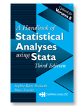
A Handbook of Statistical Analyses Using Stata, 3rd Edition

Comment from the Stata technical group

The third edition of A Handbook of Statistical Analyses Using Stata, by Sophia Rabe–Hesketh and Brian Everitt, is now available. The book provides practical examples of using Stata for real-world analysis. It begins with a concise 38-page introduction to Stata and progresses through more intermediate topics — such as multiple regression, ANOVA, and logistic regression — to more advanced topics, such as generalized linear models (GLM), survival analysis, and maximum likelihood.

New in this edition are complete chapters on cluster analysis, random-effects models, and generalized estimating equations, along with a discussion of estimating the parameters of mixed models using gllamm. (Dr. Rabe–Hesketh is the principal developer of gllamm.) The authors have also increased their emphasis on model diagnostics. Throughout the book, examples have been updated to take advantage of new features in Stata 8, particularly the new graphics capabilities.

The most distinguishing feature of this text is its use of case studies to help users learn Stata's capabilities in the various subfields of statistics, including generalized linear models, survival analysis, panel/longitudinal data, and cluster analysis. For example, the discussion of survival analysis revolves around a study of methadone maintenance treatment to aid heroin addicts in overcoming their addiction. By working with real data, the text better demonstrates the use of Stata as a problem-solving tool.

[此贴子已经被作者于2006-5-6 3:57:11编辑过]

52
hanszhu 发表于 2006-5-6 04:05:00

Stata help for xt

help xt, help iis, help tis dialogs: iis tsset -------------------------------------------------------------------------------

Title

[XT] xt -- Introduction to xt commands

Syntax

xtcmd ... [, i(varname_i) t(varname_t) ...]

iis [varname_i] [, clear]

tis [varname_i] [, clear]

Description

The xt series of commands provide tools for analyzing cross-sectional time-series datasets:

xtdes Describe pattern of xt data xtsum Summarize xt data xttab Tabulate xt data xtdata Faster specification searches with xt data

xtline Line plots with xt data

xtreg Fixed-, between- and random-effects, and population-averaged linear models xtregar Fixed- and random-effects linear models with an AR(1) disturbance xtgls Panel-data models using GLS xtpcse OLS or Prais-Winsten models with panel-corrected standard errors xtrc Random coefficients models xtivreg Instrumental variables and two-stage least squares for panel-data models xtabond Arellano-Bond linear, dynamic panel data estimator

xttobit Random-effects tobit models xtintreg Random-effects interval data regression models

xtlogit Fixed-effects, random-effects, & population-averaged logit models xtprobit Random-effects and population-averaged probit models xtcloglog Random-effects and population-averaged cloglog models

xtpoisson Fixed-effects, random-effects, & population-averaged Poisson models xtnbreg Fixed-effects, random-effects, & population-averaged negative binomial models

xtgee Population-averaged panel-data models using GEE

Cross-sectional time-series (longitudinal) datasets are of the form x_it, where x_it is a vector of observations for unti i and time t. The particular commands (such as xtdes, xtsum, xtreg, etc.) are documented in their own help file entries. This entry deals with concepts common across commands.

iis is related to the i() option on the other xt commands. Command iis or option i() sets the name of the variable corresponding to the unit index i.

tis is similarly related to the t() option. Command tis or option t() sets the name of the variable corresponding to the time index t. tis without an argument displays the current name of the time variable.

Some xt commands use time-series operators in their internal calculations, and thus require that your data be tsset; see tsset. For instance, since xtabond uses time-series operators in its internal calculations, you must tsset your data before using it. The particular help file will indicate if tsset is required before using the for the command. For these commands, iis tis are neither sufficient nor recommended.

Note that specifying iis or tis will clear any previous tsset settings. Also, specifying tsset will override any settings specified by iss or tis.

Options

i(varname_i) specifies the variable name corresponding to index i in xit. This must be a single, numeric variable, although whether it takes on the values 1, 2, 3 or 1, 7, 9, or even -2, 2^1/2, pi, is irrelevant. (If the identifying variable is a string, use egen's group() function to make a numeric variable from it; see egen.)

For instance, if the cross-sectional time-series data are of persons in the years 1991-1994, each observation is a person in one of the years; there are four observations per person (assuming no missing data). varname_i is the name of the variable that uniquely identifies the persons.

You can specify the i() option the first time you estimate, or you can use the iis command to set the i() beforehand. Note that it is not necessary to specify i() if the data have been previously tsset or if iis has been previously specified -- in these cases, the group variable is taken from the previous setting.

t(varname_t) specifies the variable name corresponding to index t in xit. This must be a single, numeric variable, although whether it takes on the values 1, 2, 3 or 1, 7, 9, or even -2, 2^1/2, pi, is irrelevant.

For instance, if the cross-sectional time-series data are of persons in the years 1991-1994, each observation is a person in one of the years; there are four observations per person (assuming no missing data). varname_t is the name of the variable that uniquely identifies the persons.

You can specify the t() option the first time you estimate, or you can use the tis command to set the t() beforehand. Note that it is not necessary to specify t() if the data have been previously tsset or if tis has been previously specified -- in these cases, the group variable is taken from the previous setting.

clear removes the definition of i() or t(). For instance, typing tis, clear makes Stata forget the identity of the t() variable.

Remarks

Once i() and t() have been specified, either by option or by the iis and tis commands, they need not be specified again except to change the variable's identity.

iis and tis, without arguments, list the current name of the index variable.

Example

An xt dataset:

pid yr_visit fev age sex height smokes ---------------------------------------------- 1071 1991 1.21 25 1 69 0 1071 1992 1.52 26 1 69 0 1071 1993 1.32 28 1 68 0 1072 1991 1.33 18 1 71 1 1072 1992 1.18 20 1 71 1 1072 1993 1.19 21 1 71 0

The other xt commands need to know the identities of the variables identifying patient and time. You could type

. iis pid . tis yr_visit

Also see

Manual: [XT] xt

Online: xtabond, xtcloglog, xtdata, xtdes, xtfrontier, xtgee, xtgls, xthtaylor, xtintreg, xtivreg, xtlogit, xtnbreg, xtpcse, xtpoisson, xtprobit, xtrc, xtreg, xtregar, xtsum, xttab, xttobit; tsset

53
hanszhu 发表于 2006-5-6 04:06:00

Stata help for time

help time -------------------------------------------------------------------------------

Title

[TS] time series -- Introduction to time-series commands}

Description

Some Stata commands are written directly for performing time-series analyses. This entry provides an index to these commands.

Many other Stata commands allow time-series operators in expressions and varlists (e.g., regress, summarize, graph, list, ...). See varlist for a table of time-series operators.

Before using time-series analysis commands or time-series operators, you must declare your data to be time series and indicate the time variable. This is done using the tsset command; see tsset.

If your interest is in analyzing cross-sectional time-series (panel) datasets, see xt.

Data management tools and time-series operators

haver Load data from Haver Analytics database tsset Declare a dataset to be time-series data tsfill Fill in missing times with missing observations in time-series data tsappend Add observations to a time-series dataset tsreport Report time-series aspects of a dataset or estimation sample tsrevar Time-series operator programming command

Univariate time-series

Estimators

arima Autoregressive integrated moving-average models arch Autoregressive conditional heteroskedasticity (ARCH) family of estimators newey Regression with Newey-West standard errors prais Prais-Winsten regression and Cochrane-Orcutt regression

Time-series smoothers and filters

tssmooth ma Moving-average filter tssmooth dexponential Double-exponential smoothing tssmooth exponential Single-exponential smoothing tssmooth hwinters Holt-Winters nonseasonal smoothing tssmooth shwinters Holt-Winters seasonal smoothing tssmooth nl Nonlinear filter

Diagnostic tools

corrgram Tabulate and graph autocorrelations xcorr Cross-correlogram for bivariate time series cumsp Cumulative spectral distribution pergram Periodogram dfgls DF-GLS unit-root test dfuller Augmented Dickey-Fuller unit-root test pperron Phillips-Perron unit-roots test dwstat Durbin-Watson d statistic durbina Durbin's alternative test for serial correlation bgodfrey Breusch-Godfrey test for higher-order serial correlation archlm Engle's LM test for the presence of autoregressive conditional heteroskedasticity wntestb Bartlett's periodogram-based test for white noise wntestq Portmanteau (Q) test for white noise

Multivariate time series

Estimators

var Vector autoregression models svar Structural vector autoregression models varbasic Fit a simple VAR and graph impulse-response functions vec Vector error-correction models

Diagnostic tools

varlmar Obtain LM statistics for residual autocorrelation after var or svar varnorm Test for normally distributed disturbances after var or svar varsoc Obtain lag-order selection statistics for VARs and VECMs varstable Check the stability condition of VAR or SVAR estimates varwle Obtain Wald lag-exclusion statistics after var or svar veclmar Obtain LM statistics for residual autocorrelation after vec vecnorm Test for normally distributed disturbances after vec vecrank Estimate the cointegrating rank using Johansen's framework vecstable Check the stability condition of VECM estimates

Forecasting, inference, and interpretation

irf create Obtain impulse-response functions and FEVDs fcast compute Compute dynamic forecasts of dependent variables after var, svar, or vec vargranger Perform pairwise Granger causality tests after var or svar

Graphs and tables

irf graph Graph impulse-response functions and FEVDs irf cgraph Combine graphs of impulse-response functions and FEVDs irf ograph Graph overlaid impulse-response functions and FEVDs irf table Create tables of impulse-response functions and FEVDs irf ctable Combine tables of impulse-response functions and FEVDs fcast graph Graph forecasts of dependent variables computed by fcast compute

Results management tools

irf add Add IRF results from one IRF file to another irf describe Describe an IRF file irf drop Drop IRF results from the active IRF file irf rename Rename an IRF result in an IRF file irf set Set the active IRF file

Also see

Manual: [U] 12.5.4 Time-series formats, [U] 24.3 Time-series dates, [U] 26.13 Models with time-series data, [TS] intro, [TS] time series

Online: tdates, tfmt, tsset, varlist, xt; and list above

54
hanszhu 发表于 2006-5-6 04:08:00

Stata Web Books
Regression with Stata
by Xiao Chen, Philip B. Ender, Michael Mitchell & Christine Wells (in alphabetical order)

The aim of these materials is to help you increase your skills in using regression analysis with Stata. This web book does not teach regression, per se, but focuses on how to perform regression analyses using Stata. It is assumed that you have had at least a one quarter/semester course in regression (linear models) or a general statistical methods course that covers simple and multiple regression and have access to a regression textbook that explains the theoretical background of the materials covered in these chapters. These materials also assume you are familiar with using Stata, for example that you have taken the ATS Stata 1 & Stata 2 classes or have equivalent knowledge of Stata. If you are a member of the UCLA community and have questions about these materials, we welcome you to send questions via email to ATSstat@ucla.edu or to visit our consulting services .

Book Chapters (also see short outline)

Accessing the Data Files. All data files used in the book are available as Stata (.dta) files. The files can be downloaded from within Stata. The general form of the command looks as follows:

    . use http://www.ats.ucla.edu/stat/stata/webbooks/reg/filename

where filename is replaced by the name of the file. Once you have loaded the data file into your computer's memory, you should save it to the local hard disk so that it will load faster when you use the file in the future. For convenience, here is a link to a zipped file which contain all the data files used in the book.

Recommended Readings

Stata Manuals. It is important to have Stata manuals to learn about the Stata commands. We hope these chapters will introduce you to a number of new Stata commands, however it is important to have the manuals to show you the detail of the syntax of the commands, examples, and technical explanations of what the commands are doing. (The help command is very useful as a quick reminder about how to use a command, but is no substitute for learning fine details of Stata commands).

For the economy minded, the Stata Reference Manual Extract is a condensed version of the reference manual that covers most of the important material for the most commonly used commands. However, if you are a serious Stata user, we recommend that you have the Stata Reference Manual (volumes 1-4) which cover all of the Stata commands in great detail. Stata manuals can be purchased at reduced rates (GradPlan pricing) for UCLA students and employees. Orders should be placed directly with Stata (how to purchase) and will be available for pick-up from Software Central within 2 business days--you will receive email notification when your purchase is ready.

Regression Textbooks. There may be a number of regression concepts introduced in the chapters that are new to you. Since the chapters focus on how to analyze your data using Stata (and not the underlying concepts) you may want to have a good regression textbook to help explain such concepts. Below we list a number of regression books that we would recommend. Each of these books is very good in their own way and yet, each one of them is different. Different individuals prefer different books from the list, and some of them may appeal to your learning style more than others. If you are interested in acquiring one of these books, we would invite you to preview them via our Statistics Books for Loan program.

Chatterjee, S., Hadi, A., & Price, B. (2000) Regression analysis by example. New York: Wiley. ISBN 0-471-31946-5

Fox, J. (1997) Applied regression analysis, linear models, and related methods. Thousand Oaks, CA: Sage Publications. ISBN 0-8039-4540-X

Hamilton, L.C. (1992) Regression with graphics. Belmont, CA: Wadsworth. ISBN 0-534-15900-1

Pedhazur, E.J. (1997). Multiple regression in behavioral research, third edition. New York: Harcourt Brace College Publishers. ISBN 0-03-072831-2

Additional Web Pages

See the Stata Topics: Regression page for additional readings and resources on regression analysis in Stata.

55
hanszhu 发表于 2006-5-6 04:08:00

Stata help for anova

help anova dialog: anova also see: anova postestimation -------------------------------------------------------------------------------

Title

[R] anova -- Analysis of variance and covariance

Syntax

anova varname [term [/] [term [/] ...]] [if] [in] [weight] [, options]

where term is of the form varname[{*||}varname[...]]

options description ------------------------------------------------------------------------- Model category(varlist) variables in terms that are categorical or class class(varlist) synonym for category(varlist) continuous(varlist) variables in terms that are continuous repeated(varlist) variables in terms that are repeated-measures variables partial use partial (or marginal) sums of squares sequential use sequential sums of squares noconstant suppress constant term

Adv. model bse(term) between-subjects error term in repeated-measures ANOVA bseunit(varname) variable representing lowest unit in the between-subjects error term grouping(varname) grouping variable for computing pooled covariance matrix

Reporting regress display the regression table [no]anova display or suppress the ANOVA table detail show mapping from values to level numbers for categorical variables ------------------------------------------------------------------------- by is allowed; see prefix. aweights and fweights are allowed; see weight. See anova postestimation for features available after estimation.

Description

The anova command fits analysis-of-variance (ANOVA) and analysis-of-covariance (ANCOVA) models for balanced and unbalanced designs, including designs with missing cells; for repeated-measures ANOVA; and for factorial, nested, or mixed designs. anova can also be used to produce regression estimates by those who have no interest in ANOVA and ANCOVA output.

If you want to fit one-way ANOVA models, you may find the oneway or loneway commands more convenient; see oneway and loneway. If you are interested in MANOVA or MANCOVA, see manova.

Options

+-------+ ----+ Model +------------------------------------------------------------

category(varlist) indicates the names of the variables in the terms that are categorical or class variables. Stata ordinarily assumes that all variables are categorical variables, so, in most cases, this option need not be specified. If you specify this option, however, the variables referenced in the terms that are not listed in category() are assumed to be continuous. Also see the class() and continuous() options.

class(varlist) is a synonym for category(varlist).

continuous(varlist) indicates the names of the variables in the terms that are continuous. Stata ordinarily assumes that all variables are categorical variables. Also see the category() and class() options.

repeated(varlist) indicates the names of the categorical variables in the terms that are to be treated as repeated-measures variables in a repeated-measures ANOVA or ANCOVA.

partial presents the ANOVA table using partial (or marginal) sums of squares. This is the default. Also see the sequential option.

sequential presents the ANOVA table using sequential sums of squares.

noconstant suppresses the constant term (intercept) from the ANOVA or regression model.

+------------+ ----+ Adv. model +-------------------------------------------------------

bse(term) indicates the between-subjects error term in a repeated-measures ANOVA. This option is needed only in the rare case when the anova command cannot automatically determine the between-subjects error term.

bseunit(varname) indicates the variable representing the lowest unit in the between-subjects error term in a repeated-measures ANOVA. This option is rarely needed since the anova command automatically selects the first variable listed in the between-subjects error term as the default for this option.

grouping(varname) indicates a variable that determines which observations are grouped together in computing the covariance matrices that will be pooled together and used in a repeated-measures ANOVA. This option is rarely needed since the anova command automatically selects the combination of all variables except the first (or as specified in the bseunit() option) in the between-subjects error term as the default for grouping observations.

+-----------+ ----+ Reporting +--------------------------------------------------------

regress presents the regression output corresponding to the specified model. Specifying regress implies the noanova option, so if you want both the regression output and ANOVA table, you must also specify the anova option. You need not specify the regress option at the time of estimation. You can obtain the underlying regression estimates at any time by typing anova, regress.

[no]anova indicates that the ANOVA table be or not be displayed. The anova command typically displays the ANOVA table, and in those cases, the noanova option suppresses the display. For instance, typing anova, detail noanova would show the detail output for the last ANOVA model while suppressing the ANOVA table itself.

If you specify the regress option, the ANOVA table is automatically suppressed. In that case, also specifying the anova option would show both the regression output and the ANOVA table.

detail presents a table showing the actual values of the categorical variables along with their mapping into level numbers. You do not have to specify this option at the time of estimation. You can obtain the output at any time by typing anova, detail.

Examples

. anova y a . anova y a b . anova y a b a*b . anova y a b c . anova y a b c a*b a*c b*c . anova y a b c a*b a*c b*c a*b*c

ANCOVA examples

. anova y a b x, continuous(x) . anova y a b x z, continuous(x z) . anova y a b x a*x a*x*x, continuous(x) . anova y a b a*b x a*x z a*z, continuous(x z)

Nested ANOVA examples

. anova output machine / operator|machine / . anova response t / c|t / d|c|t / p|d|c|t /

Split-plot ANOVA example

. anova y pr / cl|pr sk pr*sk / cl*sk|pr / gr|cl*sk|pr /

Repeated measures ANOVA examples

. anova score person drug, repeated(drug) . anova y sub / rep|sub region / region*sub / , repeated(region) . anova y cal / sub|cal shape cal*shape , repeated(shape) . anova y n / sub|n p n*p / p*sub|n d n*d / d*sub|n p*d n*p*d, rep(p d)

Also see

Manual: [R] anova

Online: anova_postestimation; encode, reshape, loneway, oneway, regress, manova

56
hanszhu 发表于 2006-5-6 04:11:00

Stata help for clogit

help clogit dialog: clogit also see: clogit postestimation -------------------------------------------------------------------------------

Title

[R] clogit -- Conditional (fixed-effects) logistic regression

Syntax

clogit depvar [indepvars] [if] [in] [weight] , group( varname) [options]

options description ------------------------------------------------------------------------- Model * group(varname) matched group variable offset(varname) include varname in model with coefficient constrained to 1 constraints(constraints) apply specified linear constraints

SE/Robust vce(vcetype) vcetype may be oim, robust, opg, bootstrap, or jackknife robust synonym for vce(robust) cluster(varname) adjust standard errors for intragroup correlation

Reporting level(#) set confidence level; default is level(95) or report odds ratios

Max options maximize_options control the maximization process; seldom used ------------------------------------------------------------------------- * group(varname) is required. bootstrap, by, jackknife, nestreg, rolling, statsby, stepwise, and xi are allowed; see prefix. fweights and iweights are allowed; see weight, but they are interpreted to apply to groups as a whole, not to individual observations. See clogit postestimation for features available after estimation.

Description

clogit fits what biostatisticians and epidemiologists call conditional logistic regression for matched case-control groups and what economists and other social scientists call fixed-effects logit for panel data. It also fits McFadden's choice model. Computationally, these models are exactly the same.

See logistic estimation commands for a list of related estimation commands.

Options

+-------+ ----+ Model +------------------------------------------------------------

group(varname) is required; it specifies an identifier variable (numeric or string) for the matched groups. strata(varname) is a synonym for group().

offset(varname); see estimation options.

constraints(numlist); see estimation options.

+-----------+ ----+ SE/Robust +--------------------------------------------------------

vce(vcetype); see vce_option.

robust, cluster(varname); see estimation options.

+-----------+ ----+ Reporting +--------------------------------------------------------

level(#); see estimation options.

or reports the estimated coefficients transformed to odds ratios, i.e., exp(b) rather than b. Standard errors and confidence intervals are similarly transformed. This option affects how results are displayed, not how they are estimated. or may be specified at estimation or when replaying previously estimated results.

+-------------+ ----+ Max options +------------------------------------------------------

maximize_options: difficult, technique(algorithm_spec), iterate(#), [no]log, trace, hessian, gradient, showstep, tolerance(#), ltolerance(#), gtolerance(#), nrtolerance(#), nonrtolerance, from(init_specs); see maximize. These options are seldom used.

Examples

Matched case-control data

. clogit low lwt nonwhite smoke ptd, group(pairid)

. clogit low lwt nonwhite smoke ptd, group(groupid)

. clogit low lwt nonwhite smoke ptd, group(groupid) or

Fixed-effects logit

. clogit union age grade not_smsa, group(idcode)

McFadden's choice model

. clogit promoted tenureb fracatt female, group(poolid)

Also see

Manual: [R] clogit

Online: clogit postestimation; cloglog, constraint, logistic, logit, mlogit, nlogit, ologit, oprobit, probit, scobit, xtcloglog, xtgee, xtlogit, xtprobit

57
hanszhu 发表于 2006-5-6 04:17:00

Stata help for multivariate

help multivariate -------------------------------------------------------------------------------

Title

[MV] multivariate -- Introduction to multivariate commands

Description

This overview organizes and presents the multivariate commands conceptually, that is, according to the similarities in the functions that they perform.

The help files listed under the heading Cluster analysis give an introduction to commands that perform cluster analysis on variables or the similarity or dissimilarity values within a matrix.

The commands listed under the heading Factor analysis and principal component analysis provide factor analysis of a correlation matrix and principal component analysis (PCA) of a correlation or covariance matrix. The correlation or covariance matrix can be provided directly or computed from variables.

The commands listed under the heading Rotation provide methods for rotating a factor or PCA solution or for rotating a matrix. Also provided is Procrustean rotation analysis for rotating a set of variables to best match another set of variables.

The commands listed under Multivariate analysis of variance and related techniques provide canonical correlation analysis, multivariate regression, multivariate analysis of variance (MANOVA), and comparison of multivariate means.

The commands listed under Multidimensional scaling and biplots provide classic MDS and two-dimensional biplots. MDS can be performed on the variables or on proximity data in a matrix or as proximity data in long format.

The commands listed under Correspondence analysis provide simple correspondence analysis (CA) on the cross-tabulation of two categorical variables or on a matrix.

Cluster analysis

* cluster Introduction to cluster analysis commands * clustermat Introduction to clustermat commands matrix dissimilarity Compute similarity or dissimilarity measures; may be used by clustermat * Contains a list of commands

Factor analysis and principal component analysis

factor Factor analysis factor postestimation Postestimation tools for factor and factormat pca Principal component analysis pca postestimation Postestimation tools for pca and pcamat rotate Orthogonal and oblique rotations after factor and pca screeplot Scree plot of eigenvalues scoreplot Score and loading plots after factor and pca

Rotation

rotate Orthogonal and oblique rotations after factor and pca rotatemat Orthogonal and oblique rotation of a Stata matrix procrustes Procrustes transformation procrustes postestimation Postestimation tools for procrustes

Multivariate analysis of variance and related techniques

canon Canonical correlations canon postestimation Postestimation tools for canon mvreg Multivariate regression mvreg postestimation Postestimation tools for mvreg manova Multivariate analysis of variance and covariance manova postestimation Postestimation tools for manova hotelling Hotelling's T-squared generalized means test

Multidimensional scaling and biplots

mds Multidimensional scaling for twoway data mds postestimation Postestimation tools for mds, mdsmat, and mdslong mdslong Multidimensional scaling of proximity data in long format mdsmat Multidimensional scaling of proximity data in a matrix biplot Biplots

Correspondence analysis

ca Simple correspondence analysis ca postestimation Postestimation tools for ca and camat

Also see

Manual: [MV] multivariate

Online: cluster, clustermat, matrix dissimilarity, factor, factor postestimation, pca, pca postestimation, rotate, screeplot, scoreplot, rotatemat, procrustes, procrustes postestimation, canon, canon postestimation, mvreg, mvreg postestimation, manova, manova postestimation, hotelling, mds, mds postestimation, mdslong, mdsmat, biplot, ca, ca postestimation

58
maoxinshu 发表于 2006-5-6 11:38:00

生成2阶以上的滞后项

gen y_2=l2.y

gen y_3=l3.y

Statachen,上面的书你都有电子版?你有Maximum Likelihood Estimation with Stata, 急需阿

59
Nicolle 学生认证  发表于 2006-5-6 12:37:00
提示: 作者被禁止或删除 内容自动屏蔽

60
Nicolle 学生认证  发表于 2006-5-6 12:38:00
提示: 作者被禁止或删除 内容自动屏蔽

您需要登录后才可以回帖 登录 | 我要注册

本版微信群
加好友,备注jltj
拉您入交流群
GMT+8, 2025-12-24 22:06