实例 | 分析38万条数据，分析保险行业中的数据应用

是 否 +2 论坛币

k人 参与回答

经管之家送您一份

应届毕业生专属福利!

求职就业群

赵安豆老师微信：zhaoandou666

经管之家联合CDA

送您一个全额奖学金名额~ !

立即领取

感谢您参与论坛问题回答

经管之家送您两个论坛币！

+2 论坛币

CDA数据分析师 出品 编辑：Mika

今天的内容是一期Python实战训练，我们来手把手教你用Python分析保险产品交叉销售和哪些因素有关。

01实战背景

首先介绍下实战的背景：

这次的数据集来自kaggle：

https://www.kaggle.com/anmolkumar/health-insurance-cross-sell-prediction

我们的客户是一家保险公司，最近新推出了一款汽车保险。现在他们的需要是建立一个模型，用来预测去年的投保人是否会对这款汽车保险感兴趣。

我们知道，保险单指的是，保险公司承诺为特定类型的损失、损害、疾病或死亡提供赔偿保证，客户则需要定期向保险公司支付一定的保险费。

这里再进一步说明一下。

例如，你每年要为20万的健康保险支付2000元的保险费。那么你肯定会想，保险公司只收取5000元的保费，这种情况下，怎么能承担如此高的住院费用呢? 这时，“概率”的概念就出现了。例如，像你一样，可能有100名客户每年支付2000元的保费，但当年住院的可能只有少数人，(比如2-3人)，而不是所有人。通过这种方式，每个人都分担了其他人的风险。

和医疗保险一样，买了车险的话，每年都需要向保险公司支付一定数额的保险费，这样在车辆发生意外事故时，保险公司将向客户提供赔偿（称为“保险金额”）。

我们要做的就是建立模型，来预测客户是否对汽车保险感兴趣。这对保险公司来说是非常有帮助的，公司可以据此制定沟通策略，接触这些客户，并优化其商业模式和收入。

02数据理解

为了预测客户是否对车辆保险感兴趣，我们需要了解一些客户信息 (性别、年龄等)、车辆(车龄、损坏情况)、保单(保费、采购渠道)等信息。

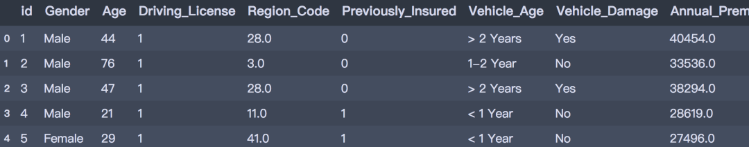
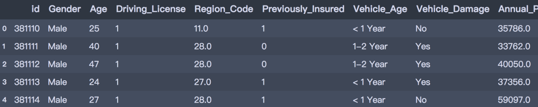
数据划分为训练集和测试集，训练数据包含381109笔客户资料，每笔客户资料包含12个字段，1个客户ID字段、10个输入字段及1个目标字段-Response是否响应(1代表感兴趣，0代表不感兴趣)。测试数据包含127037笔客户资料；字段个数与训练数据相同，目标字段没有值。字段的定义可参考下文。

下面我们开始吧！

03数据读入和预览

首先开始数据读入和预览。

1. # 数据整理
   
2. import numpy as np
   
3. import pandas as pd
   
4. 
   
5. # 可视化
   
6. import matplotlib.pyplot as plt
   
7. import seaborn as sns
   
8. import plotly as py
   
9. import plotly.graph_objs as go
   
10. import plotly.express as px
    
11. pyplot = py.offline.plot
    
12. from exploratory_data_analysis import EDAnalysis # 自定义

复制代码

1. # 读入训练集
   
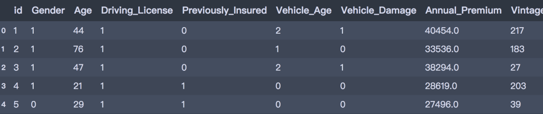
2. train = pd.read_csv('../data/train.csv')
   
3. train.head()

复制代码

1. # 读入测试集
   
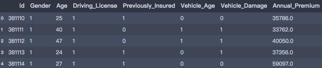
2. test = pd.read_csv('../data/test.csv')
   
3. test.head()

复制代码

1. print(train.info())
   
2. print('-' * 50)
   
3. print(test.info())

复制代码

1. <class 'pandas.core.frame.DataFrame'>
   
2. RangeIndex: 381109 entries, 0 to 381108
   
3. Data columns (total 12 columns):
   
4. #   Column                Non-Null Count   Dtype  
   
5. ---  ------                --------------   -----  
   
6. 0   id                    381109 non-null  int64  
   
7. 1   Gender                381109 non-null  object
   
8. 2   Age                   381109 non-null  int64  
   
9. 3   Driving_License       381109 non-null  int64  
   
10. 4   Region_Code           381109 non-null  float64
    
11. 5   Previously_Insured    381109 non-null  int64  
    
12. 6   Vehicle_Age           381109 non-null  object
    
13. 7   Vehicle_Damage        381109 non-null  object
    
14. 8   Annual_Premium        381109 non-null  float64
    
15. 9   Policy_Sales_Channel  381109 non-null  float64
    
16. 10  Vintage               381109 non-null  int64  
    
17. 11  Response              381109 non-null  int64  
    
18. dtypes: float64(3), int64(6), object(3)
    
19. memory usage: 34.9+ MB
    
20. None
    
21. --------------------------------------------------
    
22. <class 'pandas.core.frame.DataFrame'>
    
23. RangeIndex: 127037 entries, 0 to 127036
    
24. Data columns (total 11 columns):
    
25. #   Column                Non-Null Count   Dtype  
    
26. ---  ------                --------------   -----  
    
27. 0   id                    127037 non-null  int64  
    
28. 1   Gender                127037 non-null  object
    
29. 2   Age                   127037 non-null  int64  
    
30. 3   Driving_License       127037 non-null  int64  
    
31. 4   Region_Code           127037 non-null  float64
    
32. 5   Previously_Insured    127037 non-null  int64  
    
33. 6   Vehicle_Age           127037 non-null  object
    
34. 7   Vehicle_Damage        127037 non-null  object
    
35. 8   Annual_Premium        127037 non-null  float64
    
36. 9   Policy_Sales_Channel  127037 non-null  float64
    
37. 10  Vintage               127037 non-null  int64  
    
38. dtypes: float64(3), int64(5), object(3)
    
39. memory usage: 10.7+ MB
    
40. None

复制代码

04探索性分析

下面，我们基于训练数据集进行探索性数据分析。

1. 描述性分析

首先对数据集中数值型属性进行描述性统计分析。

1. desc_table = train.drop(['id', 'Vehicle_Age'], axis=1).describe().T
   
2. desc_table

复制代码

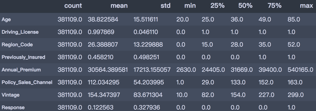
通过描述性分析后，可以得到以下结论。

从以上描述性分析结果可以得出：

• 客户年龄：客户的年龄范围在20 ~ 85岁之间，平均年龄是38岁，青年群体居多；
• 是否有驾照：99.89%客户都持有驾照；
• 之前是否投保：45.82%的客户已经购买了车辆保险；
• 年度保费：客户的保费范围在2630 ~ 540165之间，平均的保费金额是30564。
• 往来时长：此数据基于过去一年的数据，客户的往来时间范围在10~299天之间，平均往来时长为154天。
• 是否响应：平均来看，客户对车辆保险感兴趣的概率为12.25%。
  
  

2. 目标变量的分布

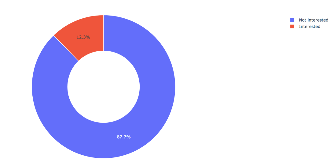
训练集共有381109笔客户资料，其中感兴趣的有46710人，占比12.3%，不感兴趣的有334399人，占比87.7%。

1. train['Response'].value_counts()
   
2. 0    334399
   
3. 1     46710
   
4. Name: Response, dtype: int64

复制代码

1. values = train['Response'].value_counts().values.tolist()
   
2. 
   
3. # 轨迹
   
4. trace1 = go.Pie(labels=['Not interested', 'Interested'],
   
5.                 values=values,
   
6.                 hole=.5,
   
7.                 marker={'line': {'color': 'white', 'width': 1.3}}
   
8.                )
   
9. # 轨迹列表
   
10. data = [trace1]
    
11. # 布局
    
12. layout = go.Layout(title=f'Distribution_ratio of Response', height=600)
    
13. # 画布
    
14. fig = go.Figure(data=data, layout=layout)
    
15. # 生成HTML
    
16. pyplot(fig, filename='./html/目标变量分布.html')

复制代码

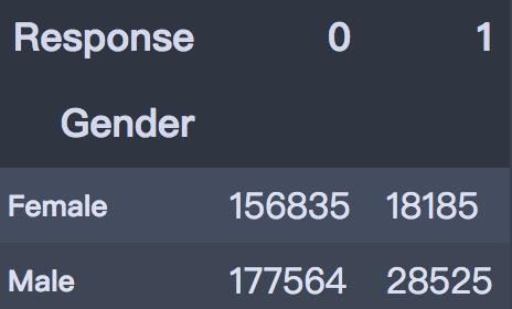
3. 性别因素

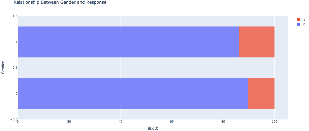
从条形图可以看出，男性的客户群体对汽车保险感兴趣的概率稍高，是13.84%，相较女性客户高出3个百分点。

1. pd.crosstab(train['Gender'], train['Response'])  

复制代码

1. # 实例类
   
2. eda = EDAnalysis(data=train, id_col='id', target='Response')
   
3. 
   
4. # 柱形图
   
5. fig = eda.draw_bar_stack_cat(colname='Gender')
   
6. pyplot(fig, filename='./html/性别与是否感兴趣.html')

复制代码

4. 之前是否投保

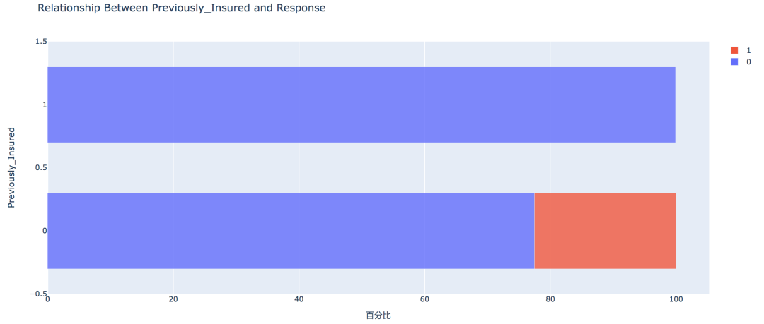
没有购买汽车保险的客户响应概率更高，为22.54%，有购买汽车保险的客户则没有这一需求，感兴趣的概率仅为0.09%。

1. pd.crosstab(train['Previously_Insured'], train['Response'])  

复制代码

1. fig = eda.draw_bar_stack_cat(colname='Previously_Insured')
   
2. pyplot(fig, filename='./html/之前是否投保与是否感兴趣.html')  

复制代码

5. 车龄因素

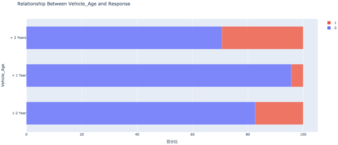
车龄越大，响应概率越高，大于两年的车龄感兴趣的概率最高，为29.37%，其次是1~2年车龄，概率为17.38%。小于1年的仅为4.37%。

6. 车辆损坏情况

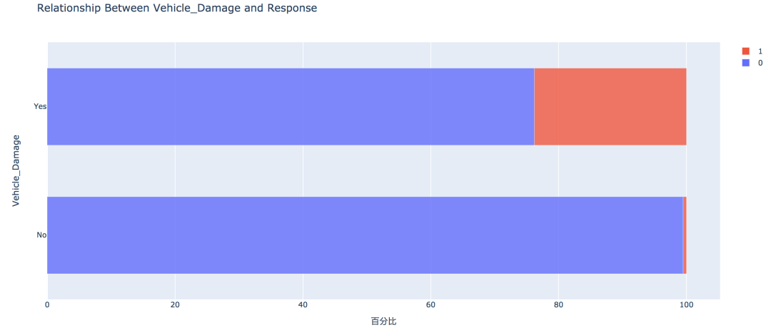
车辆曾经损坏过的客户有较高的响应概率，为23.76%，相比之下，客户过去车辆没有损坏的响应概率仅为0.52%

7. 不同年龄

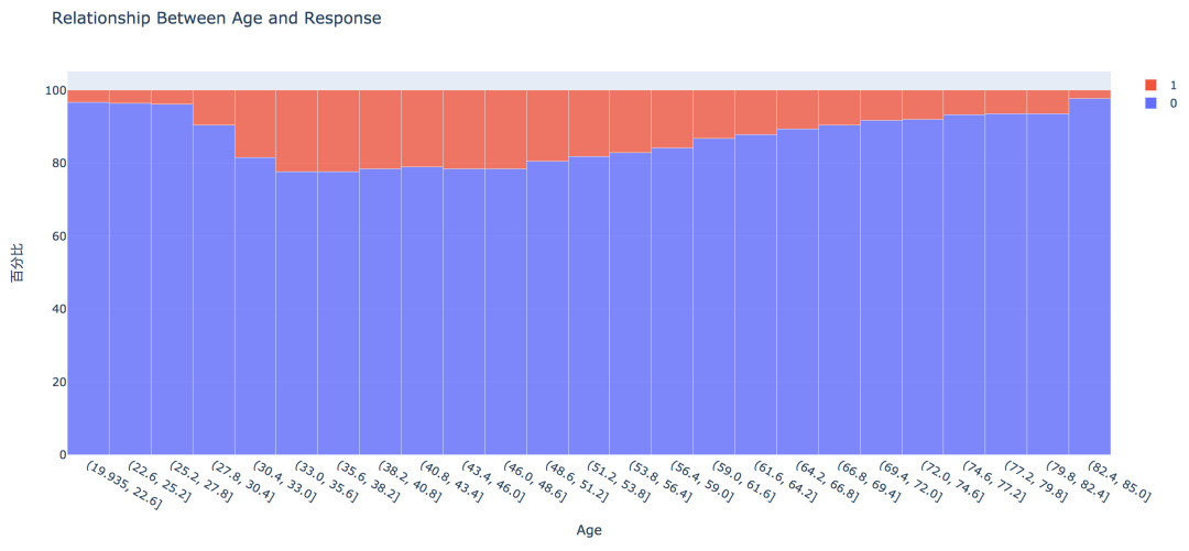
从直方图中可以看出，年龄较高的群体和较低的群体响应的概率较低，30~60岁之前的客户响应概率较高。

通过可视化探索，我们大致可以知道:

车龄在1年以上，之前有车辆损坏的情况出现，且未购买过车辆保险的客户有较高的响应概率。

05数据预处理

此部分工作主要包含字段选择，数据清洗和数据编码，字段的处理如下：

• Region_Code和Policy_Sales_Channel：分类数过多，且不易解读，删除；
• Annual_Premium：异常值处理
• Gender、Vehicle_Age、Vehicle_Damage：分类型数据转换为数值型编码
  
  

1. # 删除字段
   
2. train = train.drop(['Region_Code', 'Policy_Sales_Channel'], axis=1)
   
3. 
   
4. # 盖帽法处理异常值
   
5. f_max = train['Annual_Premium'].mean() + 3*train['Annual_Premium'].std()
   
6. f_min = train['Annual_Premium'].mean() - 3*train['Annual_Premium'].std()
   
7. 
   
8. train.loc[train['Annual_Premium'] > f_max, 'Annual_Premium'] = f_max
   
9. train.loc[train['Annual_Premium'] < f_min, 'Annual_Premium'] = f_min
   
10. 
    
11. # 数据编码
    
12. train['Gender'] = train['Gender'].map({'Male': 1, 'Female': 0})
    
13. train['Vehicle_Damage'] = train['Vehicle_Damage'].map({'Yes': 1, 'No': 0})
    
14. train['Vehicle_Age'] = train['Vehicle_Age'].map({'< 1 Year': 0, '1-2 Year': 1, '> 2 Years': 2})
    
15. train.head()

复制代码

测试集做相同的处理：

1. # 删除字段
   
2. test = test.drop(['Region_Code', 'Policy_Sales_Channel'], axis=1)  
   
3. # 盖帽法处理
   
4. test.loc[test['Annual_Premium'] > f_max, 'Annual_Premium'] = f_max
   
5. test.loc[test['Annual_Premium'] < f_min, 'Annual_Premium'] = f_min
   
6. 
   
7. # 数据编码
   
8. test['Gender'] = test['Gender'].map({'Male': 1, 'Female': 0})
   
9. test['Vehicle_Damage'] = test['Vehicle_Damage'].map({'Yes': 1, 'No': 0})
   
10. test['Vehicle_Age'] = test['Vehicle_Age'].map({'< 1 Year': 0, '1-2 Year': 1, '> 2 Years': 2})
    
11. test.head()

复制代码

06数据建模

我们选择使用以下几种模型进行建置，并比较模型的分类效能。

首先在将训练集划分为训练集和验证集，其中训练集用于训练模型，验证集用于验证模型效果。首先导入建模库：

1. # 建模
   
2. from sklearn.linear_model import LogisticRegression
   
3. from sklearn.neighbors import KNeighborsClassifier
   
4. from sklearn.tree import DecisionTreeClassifier
   
5. from sklearn.ensemble import RandomForestClassifier
   
6. from lightgbm import LGBMClassifier
   
7. 
   
8. # 预处理
   
9. from sklearn.preprocessing import StandardScaler, MinMaxScaler
   
10. 
    
11. # 模型评估
    
12. from sklearn.model_selection import train_test_split, GridSearchCV
    
13. from sklearn.metrics import confusion_matrix, classification_report, accuracy_score, f1_score, roc_auc_score

复制代码

1. # 划分特征和标签
   
2. X = train.drop(['id', 'Response'], axis=1)
   
3. y = train['Response']
   
4. 
   
5. # 划分训练集和验证集(分层抽样)
   
6. X_train, X_val, y_train, y_val = train_test_split(X, y, test_size=0.2, stratify=y, random_state=0)
   
7. print(X_train.shape, X_val.shape, y_train.shape, y_val.shape)
   
8. (304887, 8) (76222, 8) (304887,) (76222,)

复制代码

1. # 处理样本不平衡，对0类样本进行降采样
   
2. from imblearn.under_sampling import RandomUnderSampler
   
3. 
   
4. under_model = RandomUnderSampler(sampling_strategy={0:133759, 1:37368}, random_state=0)
   
5. X_train, y_train = under_model.fit_sample(X_train, y_train)  
   
6. # 保存一份极值标准化的数据
   
7. mms = MinMaxScaler()
   
8. 
   
9. X_train_scaled = pd.DataFrame(mms.fit_transform(X_train), columns=x_under.columns)
   
10. X_val_scaled = pd.DataFrame(mms.transform(X_val), columns=x_under.columns)
    
11. 
    
12. # 测试集
    
13. X_test = test.drop('id', axis=1)
    
14. X_test_scaled = pd.DataFrame(mms.transform(X_test), columns=X_test.columns)

复制代码

1. KNN算法

1. # 建立knn
   
2. knn = KNeighborsClassifier(n_neighbors=3, n_jobs=-1)
   
3. knn.fit(X_train_scaled, y_train)
   
4. 
   
5. y_pred = knn.predict(X_val_scaled)
   
6. 
   
7. print('Simple KNeighborsClassifier accuracy：%.3f' % (accuracy_score(y_val, y_pred)))
   
8. print('Simple KNeighborsClassifier f1_score: %.3f' % (f1_score(y_val, y_pred)))  
   
9. print('Simple KNeighborsClassifier roc_auc_score: %.3f' % (roc_auc_score(y_val, y_pred)))

复制代码

1. Simple KNeighborsClassifier accuracy：0.807
   
2. Simple KNeighborsClassifier f1_score: 0.337
   
3. Simple KNeighborsClassifier roc_auc_score: 0.632

复制代码

1. # 对测试集评估
   
2. test_y = knn.predict(X_test_scaled)
   
3. test_y[:5]
   
4. array([0, 0, 1, 0, 0], dtype=int64)

复制代码

2. Logistic回归

1. # Logistic回归
   
2. lr = LogisticRegression()
   
3. lr.fit(X_train_scaled, y_train)
   
4. 
   
5. y_pred = lr.predict(X_val_scaled)
   
6. 
   
7. print('Simple LogisticRegression accuracy：%.3f' % (accuracy_score(y_val, y_pred)))
   
8. print('Simple LogisticRegression f1_score: %.3f' % (f1_score(y_val, y_pred)))  
   
9. print('Simple LogisticRegression roc_auc_score: %.3f' % (roc_auc_score(y_val, y_pred)))

复制代码

1. Simple LogisticRegression accuracy：0.863
   
2. Simple LogisticRegression f1_score: 0.156
   
3. Simple LogisticRegression roc_auc_score: 0.536

复制代码

3. 决策树

1. # 决策树
   
2. dtc = DecisionTreeClassifier(max_depth=10, random_state=0)
   
3. dtc.fit(X_train, y_train)
   
4. 
   
5. y_pred = dtc.predict(X_val)
   
6. 
   
7. print('Simple DecisionTreeClassifier accuracy：%.3f' % (accuracy_score(y_val, y_pred)))
   
8. print('Simple DecisionTreeClassifier f1_score: %.3f' % (f1_score(y_val, y_pred)))  
   
9. print('Simple DecisionTreeClassifier roc_auc_score: %.3f' % (roc_auc_score(y_val, y_pred)))

复制代码

1. Simple DecisionTreeClassifier accuracy：0.849
   
2. Simple DecisionTreeClassifier f1_score: 0.310
   
3. Simple DecisionTreeClassifier roc_auc_score: 0.603

复制代码

4. 随机森林

1. # 决策树
   
2. rfc = RandomForestClassifier(n_estimators=100, max_depth=10, n_jobs=-1)  
   
3. rfc.fit(X_train, y_train)
   
4. 
   
5. y_pred = rfc.predict(X_val)
   
6. 
   
7. print('Simple RandomForestClassifier accuracy：%.3f' % (accuracy_score(y_val, y_pred)))
   
8. print('Simple RandomForestClassifier f1_score: %.3f' % (f1_score(y_val, y_pred)))  
   
9. print('Simple RandomForestClassifier roc_auc_score: %.3f' % (roc_auc_score(y_val, y_pred)))

复制代码

1. Simple RandomForestClassifier accuracy：0.870
   
2. Simple RandomForestClassifier f1_score: 0.177
   
3. Simple RandomForestClassifier roc_auc_score: 0.545

复制代码

5. LightGBM

1. lgbm = LGBMClassifier(n_estimators=100, random_state=0)
   
2. lgbm.fit(X_train, y_train)
   
3. 
   
4. y_pred = lgbm.predict(X_val)
   
5. 
   
6. print('Simple LGBM accuracy: %.3f' % (accuracy_score(y_val, y_pred)))
   
7. print('Simple LGBM f1_score: %.3f' % (f1_score(y_val, y_pred)))  
   
8. print('Simple LGBM roc_auc_score: %.3f' % (roc_auc_score(y_val, y_pred)))

复制代码

1. Simple LGBM accuracy: 0.857
   
2. Simple LGBM f1_score: 0.290
   
3. Simple LGBM roc_auc_score: 0.591

复制代码

综上，以f1-score作为评价标准的情况下，KNN算法有较好的分类效能，这可能是由于数据样本本身不平衡导致，后续可以通过其他类别不平衡的方式做进一步处理，同时可以通过参数调整的方式来优化其他模型，通过调整预测的门槛值来增加预测效能等其他方式。

相关帖子DA内容精选 精益业务数据分析试读 CDA认证考试模拟题库及考试资料（最新版）免费获取 深度学习TensorFlow 与 PyTorch训练营试听课 统计分析轻松入门 | 张文彤老师课程系列 Python空间地理数据分析与可视化（体验课） CDA认证官网 草根数据分析师的深造之路 | CDA 持证人分享 材料专业硕士工作3年，如何转型数据分析师 | CDA 持证人分享 数据科学和企业的数据能力建设 数据分析最常用的excel函数公式大全

扫码加我 拉你入群

请注明：姓名-公司-职位

以便审核进群资格，未注明则拒绝

分享0 收藏1 回帖

关键词：保险行业 randomForest distribution Exploratory classifier