【推荐】【精品文章】Bayesian Statistics explained to Beginners in Simple

是 否 +2 论坛币

k人 参与回答

经管之家送您一份

应届毕业生专属福利!

求职就业群

赵安豆老师微信：zhaoandou666

经管之家联合CDA

送您一个全额奖学金名额~ !

立即领取

感谢您参与论坛问题回答

经管之家送您两个论坛币！

+2 论坛币

Introduction

Bayesian Statistics continues to remain incomprehensible in the ignited minds of many analysts. Being amazed by the incredible power of machine learning, a lot of us have become unfaithful to statistics. Our focus has narrowed down to exploring machine learning. Isn’t it true?

We fail to understand that machine learning is only one way to solve real world problems. In several situations, it does not help us solve business problems, even though there is data involved in these problems. To say the least, knowledge of statistics will allow you to work on complex analytical problems, irrespective of the size of data.

In 1770s, Thomas Bayes introduced ‘Bayes Theorem’. Even after centuries later, the importance of ‘Bayesian Statistics’ hasn’t faded away. In fact, today this topic is being taught in great depths in some of the world’s leading universities.

With this idea, I’ve created this beginner’s guide on Bayesian Statistics. I’ve tried to explain the concepts in a simplistic manner with examples. Prior knowledge of basic probability & statistics is desirable. By the end of this article, you will have a concrete understanding of Bayesian Statistics and its associated concepts.

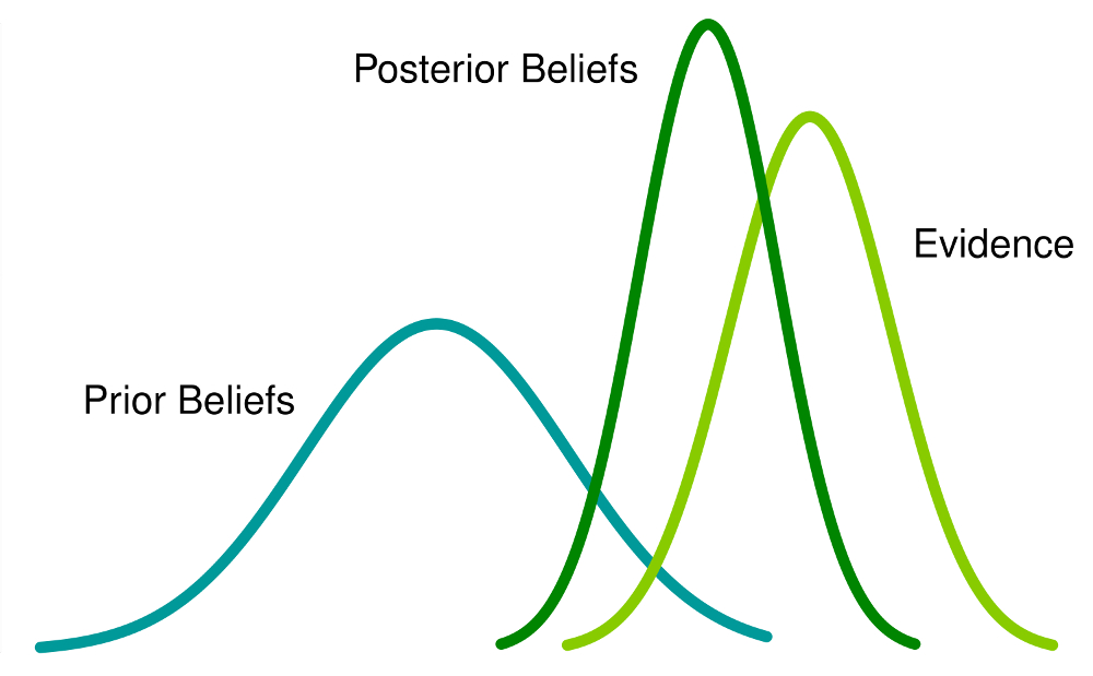
Table of Contents

• Frequentist Statistics
• The Inherent Flaws in Frequentist Statistics
• Bayesian Statistics
  
  • Conditional Probability
  • Bayes Theorem
    
• Bayesian Inference
  
  • Bernoulli likelihood function
  • Prior Belief Distribution
  • Posterior belief Distribution
    
• Test for Significance – Frequentist vs Bayesian
  
  • p-value
  • Confidence Intervals
  • Bayes Factor
  • High Density Interval (HDI)
    
  
  

Before we actually delve in Bayesian Statistics, let us spend a few minutes understanding Frequentist Statistics, the more popular version of statistics most of us come across and the inherent problems in that.

1. Frequentist Statistics

The debate between frequentist and bayesian have haunted beginners for centuries. Therefore, it is important to understand the difference between the two and how does there exists a thin line of demarcation!

It is the most widely used inferential technique in the statistical world. Infact, generally it is the first school of thought that a person entering into the statistics world comes across.

Frequentist Statistics tests whether an event (hypothesis) occurs or not. It calculates the probability of an event in the long run of the experiment (i.e the experiment is repeated under the same conditions to obtain the outcome).

Here, the sampling distributions of fixed size are taken. Then, the experiment is theoretically repeatedinfinite number of times but practically done with a stopping intention. For example, I perform an experiment with a stopping intention in mind that I will stop the experiment when it is repeated 1000 times or I see minimum 300 heads in a coin toss.

Let’s go deeper now.

Now, we’ll understand frequentist statistics using an example of coin toss. The objective is to estimate the fairness of the coin. Below is a table representing the frequency of heads:

We know that probability of getting a head on tossing a fair coin is 0.5. No. of heads represents the actual number of heads obtained. Difference is the difference between0.5*(No. of tosses) - no. of heads.

An important thing is to note that, though the difference between the actual number of heads and expected number of heads( 50% of number of tosses) increases as the number of tosses are increased, the proportion of number of heads to total number of tosses approaches 0.5 (for a fair coin).

This experiment presents us with a very common flaw found in frequentist approach i.e. Dependence of the result of an experiment on the number of times the experiment is repeated.

To know more about frequentist statistical methods, you can head to this excellent course on inferential statistics.

2. The Inherent Flaws in Frequentist Statistics

Till here, we’ve seen just one flaw in frequentist statistics. Well, it’s just the beginning.

20th century saw a massive upsurge in the frequentist statistics being applied to numerical models to check whether one sample is different from the other, a parameter is important enough to be kept in the model and variousother  manifestations of hypothesis testing. But frequentist statistics suffered some great flaws in its design and interpretation  which posed a serious concern in all real life problems. For example:

1. p-values measured against a sample (fixed size) statistic with some stopping intention changes with change in intention and sample size. i.e If two persons work on the same data and have different stopping intention, they may get two different  p- values for the same data, which is undesirable.

For example: Person A may choose to stop tossing a coin when the total count reaches 100 while B stops at 1000. For different sample sizes, we get different t-scores and different p-values. Similarly, intention to stop may change from fixed number of flips to total duration of flipping. In this case too, we are bound to get different p-values.

2- Confidence Interval (C.I) like p-value depends heavily on the sample size. This makes the stopping potential absolutely absurd since no matter how many persons perform the tests on the same data, the results should be consistent.

3- Confidence Intervals (C.I) are not probability distributions therefore they do not provide the most probable value for a parameter and the most probable values.

These three reasons are enough to get you going into thinking about the drawbacks of the frequentist approach and why is there a need for bayesian approach. Let’s find it out.

From here, we’ll first understand the basics of Bayesian Statistics.

扫码加我 拉你入群

请注明：姓名-公司-职位

以便审核进群资格，未注明则拒绝

分享0 收藏1 回帖

关键词：Statistics statistic beginners Explained Bayesian explained English

3. Bayesian Statistics

“Bayesian statistics is a mathematical procedure that applies probabilities to statistical problems. It provides people the tools to update their beliefs in the evidence of new data.”

You got that? Let me explain it with an example:

Suppose, out of all the 4 championship races (F1) between Niki Lauda and James hunt, Niki won 3 times while James managed only 1.

So, if you were to bet on the winner of next race, who would he be ?

I bet you would say Niki Lauda.

Here’s the twist. What if you are told that it rained once when James won and once when Niki won and it is definite that it will rain on the next date. So, who would you bet your money on now ?

By intuition, it is easy to see that chances of winning for James have increased drastically. But the question is: how much ?

To understand the problem at hand, we need to become familiar with some concepts, first of which is conditional probability (explained below).

In addition, there are certain pre-requisites:

Pre-Requisites:

• Linear Algebra : To refresh your basics, you can check out Khan’s Academy Algebra.
• Probability and Basic Statistics : To refresh your basics, you can check out another course by Khan Academy.
  

3.1 Conditional Probability

It is defined as the: Probability of an event A given B equals the probability of B and A happening together divided by the probability of B.”

For example: Assume two partially intersecting sets A and B as shown below.

Set A represents one set of events and Set B represents another. We wish to calculate the probability of A given B has already happened. Lets represent the happening of event B by shading it with red.

Now since B has happened, the part which now matters for A is the part shaded in blue which is interestingly . So, the probability of A given B turns out to be:

Therefore, we can write the formula for event B given A has already occurred by:

or

Now, the second equation can be rewritten as :

This is known as Conditional Probability.

Let’s try to answer a betting problem with this technique.

Suppose, B be the event of winning of James Hunt. A be the event of raining. Therefore,

• P(A) =1/2, since it rained twice out of four days.
• P(B) is 1/4, since James won only one race out of four.
• P(A|B)=1, since it rained every time when James won.
  

Substituting the values in the conditional probability formula, we get the probability to be around 50%, which is almost the double of 25% when rain was not taken into account (Solve it at your end).

This further strengthened our belief  ofJames winning in the light of new evidence i.e rain. You must be wondering that this formula bears close resemblance to something you might have heard a lot about. Think!

Probably, you guessed it right. It looks like Bayes Theorem.

Bayes  theorem is built on top of conditional probability and lies in the heart of Bayesian Inference. Let’s understand it in detail now.

3.2 Bayes Theorem

Bayes Theorem comes into effect when multiple events form an exhaustive set with another event B. This could be understood with the help of the below diagram.

Now, B can be written as

So, probability of B can be written as,

But

So, replacing P(B) in the equation of conditional probability we get

This is the equation of Bayes Theorem.

4. Bayesian Inference

There is no point in diving into the theoretical aspect of it. So, we’ll learn how it works! Let’s take an example of coin tossing to understand the idea behind bayesian inference.

An important part of bayesian inference is the establishment of parameters and models.

Models are the mathematical formulation of the observed events. Parameters are the factors in the models affecting the observed data. For example, in tossing a coin, fairness of coin may be defined as the parameter of coin denoted by θ. The outcome of the events may be denoted by D.

Answer this now. What is the probability of 4 heads out of 9 tosses(D) given the fairness of coin (θ). i.eP(D|θ)

Wait, did I ask the right question? No.

We should be more interested in knowing : Given an outcome (D) what is the probbaility of coin being fair (θ=0.5)

Lets represent it using Bayes Theorem:

P(θ|D)=(P(D|θ) X P(θ))/P(D)

Here, P(θ)is the prior i.e the strength of our belief in the fairness of coin before the toss. It is perfectly okay to believe that coin can have any degree of fairness between 0 and 1.

P(D|θ) is the likelihood of observing our result given our distribution for θ. If we knew that coin was fair, this gives the probability of observing the number of heads in a particular number of flips.

P(D) is the evidence. This is the probability of data as determined by summing (or integrating) across all possible values of θ, weighted by how strongly we believe in those particular values of θ.

If we had multiple views of what the fairness of the coin is (but didn’t know for sure), then this tells us the probability of seeing a certain sequence of flips for all possibilities of our belief in the coin’s fairness.

P(θ|D) is the posterior belief of our parameters after observing the evidence i.e the number of heads .

From here, we’ll dive deeper into mathematical implications of this concept. Don’t worry. Once you understand them, getting to its mathematics is pretty easy.

To define our model correctly , we need two mathematical models before hand. One to represent thelikelihood function P(D|θ) and the other for representing the distribution of prior beliefs . The product of these two gives the posterior belief P(θ|D) distribution.

Since prior and posterior are both beliefs about the distribution of fairness of coin, intuition tells us that both should have the same mathematical form. Keep this in mind. We will come back to it again.

So, there are several functions which support the existence of bayes theorem. Knowing them is important, hence I have explained them in detail.

4.1. Bernoulli likelihood function

Lets recap what we learned about the likelihood function. So, we learned that:

It is the probability of observing a particular number of heads in a particular number of flips for a given fairness of coin. This means our probability of observing heads/tails depends upon the fairness of coin (θ).

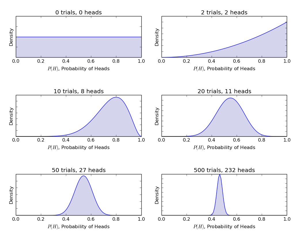
P(y=1|θ)=     [If coin is fair θ=0.5, probability of observing heads (y=1) is 0.5]

P(y=0|θ)= [If coin is fair θ=0.5, probability of observing tails(y=0) is 0.5]

It is worth noticing that representing 1 as heads and 0 as tails is just a mathematical notation to formulate a model. We can combine the above mathematical definitions into a single definition to represent the probability of both the outcomes.

P(y|θ)=

This is called the Bernoulli Likelihood Function and the task of coin flipping is called Bernoulli’s trials.

y={0,1},θ=(0,1)

And, when we want to see a series of heads or flips, its probability is given by:

Furthermore, if we are interested in the probability of number of heads z turning up in N number of flips then the probability is given by:

4.2. Prior Belief  Distribution

This distribution is used to represent our strengths on beliefs about the parameters based on the previous experience.

But, what if one has no previous experience?

Don’t worry. Mathematicians have devised methods to mitigate this problem too. It is known asuninformative priors. I would like to inform you beforehand that it is just a misnomer. Every uninformative prior always provides some information event the constant distribution prior.

Well, the mathematical function used to represent the prior beliefs is known as beta distribution. It has some very nice mathematical properties which enable us to model our beliefs about a binomial distribution.

Probability density function of beta distribution is of the form :

where, our focus stays on numerator. The denominator is there just to ensure that the total probability density function upon integration evaluates to 1.

α and β are called the shape deciding parameters of the density function. Here α is analogous to number of heads in the trials and β corresponds to the number of tails. The diagrams below will help you visualize the beta distributions for different values of α and β

You too can draw the beta distribution for yourself using the following code in R:

> library(stats)
> par(mfrow=c(3,2))
> x=seq(0,1,by=o.1)
> alpha=c(0,2,10,20,50,500)
> beta=c(0,2,8,11,27,232)
> for(i in 1:length(alpha)){
       y<-dbeta(x,shape1=alpha,shape2=beta)
       plot(x,y,type="l")
}

Note: α and β are intuitive to understand since they can be calculated by knowing the mean (μ) and standard deviation (σ) of the distribution. In fact, they are related as :

If mean and standard deviation of a distribution are known , then there shape parameters can be easily calculated.

Inference drawn from graphs above:

• When there was no toss we believed that every fairness of coin is possible as depicted by the flat line.
• When there were more number of heads than the tails, the graph showed a peak shifted towards the right side, indicating higher probability of heads and that coin is not fair.
• As more tosses are done, and heads continue to come in larger proportion the peak narrows increasing our confidence in the fairness of the coin value.
  

4.3. Posterior Belief Distribution

The reason that we chose prior belief is to obtain a beta distribution. This is because when we multiply it with a likelihood function, posterior distribution yields a form similar to the prior distribution which is much easier to relate to and understand. If this much information whets your appetite, I’m sure you are ready to walk an extra mile.

Let’s calculate posterior belief using bayes theorem.

Calculating posterior belief using Bayes Theorem

Now, our posterior belief becomes,

This is interesting. Just knowing the mean and standard distribution of our belief about the parameter θ and by observing the number of heads in N flips, we can update our belief about the model parameter(θ).

Lets understand this with the help of a simple example:

Suppose, you think that a coin is biased. It has a mean (μ) bias of around 0.6 with standard deviation of 0.1.

Then ,

α= 13.8 , β=9.2

i.e our distribution will be biased on the right side. Suppose, you observed 80 heads (z=80) in 100 flips(N=100). Let’s see how our prior and posterior beliefs are going to look:

prior = P(θ|α,β)=P(θ|13.8,9.2)

Posterior = P(θ|z+α,N-z+β)=P(θ|93.8,29.2)

Lets visualize both the beliefs on a graph:

The R code for the above graph is as:

> library(stats)
> x=seq(0,1,by=0.1)
> alpha=c(13.8,93.8)
> beta=c(9.2,29.2)
> for(i in 1:length(alpha)){
      y<-dbeta(x,shape1=alpha,shape2=beta)
      plot(x,y,type="l",xlab = "theta",ylab = "density")

}

As more and more flips are made and new data is observed, our beliefs get updated. This is the real power of Bayesian Inference.

5. Test for Significance – Frequentist vs Bayesian

Without going into the rigorous mathematical structures, this section will provide you a quick overview of different approaches of frequentist and bayesian methods to test for significance and difference between groups and which method is most reliable.

5.1. p-value

In this, the t-score for a particular sample from a sampling distribution of fixed size is calculated. Then, p-values are predicted. We can interpret p values as (taking an example of p-value as 0.02 for a distribution of mean 100) : There is 2% probability that the sample will have mean equal to 100.

This interpretation suffers from the flaw that for sampling distributions of different sizes, one is bound to get different t-score and hence different p-value. It is completely absurd. A p-value less than 5% does not guarantee that null hypothesis is wrong nor a p-value greater than 5% ensures that null hypothesis is right.

5.2. Confidence Intervals

Confidence Intervals also suffer from the same defect. Moreover since C.I is not a probability distribution , there is no way to know which values are most probable.

5.3. Bayes Factor

Bayes factor is the equivalent of p-value in the bayesian framework. Lets understand it in an comprehensive manner.

The null hypothesis in bayesian framework assumes ∞ probability distribution only at a particular value of a parameter (say θ=0.5) and a zero probability else where. (M1)

The alternative hypothesis is that all values of θ are possible, hence a flat curve representing the distribution. (M2)

Now, posterior distribution of the new data looks like below.

Bayesian statistics adjusted credibility (probability) of various values of θ. It can be easily seen that the probability distribution has shifted towards M2 with a value higher than M1 i.e M2 is more likely to happen.

Bayes factor does not depend upon the actual distribution values of θ but the magnitude of shift in values of M1 and M2.

In panel A (shown above): left bar (M1) is the prior probability of the null hypothesis.

In panel B (shown), the left bar is the posterior probability of the null hypothesis.

Bayes factor is defined as the ratio of the posterior odds to the prior odds,

To reject a null hypothesis, a BF <1/10 is preferred.

We can see the immediate benefits of using Bayes Factor instead of p-values since they are independent of intentions and sample size.

5.4. High Density Interval (HDI)

HDI is formed from the posterior distribution after observing the new data. Since HDI is a probability, the 95% HDI gives the 95% most credible values. It is also guaranteed that 95 % values will lie in this interval unlike C.I.

Notice, how the 95% HDI in prior distribution is wider than the 95% posterior distribution. This is because our belief in HDI increases upon observation of new data.

End Notes

The aim of this article was to get you thinking about the different type of statistical philosophies out there and how any single of them cannot be used in every situation.

It’s a high time that both the philosophies are merged to mitigate the real world problems by addressing the flaws of the other. Part II of this series will focus on the Dimensionality Reduction techniques using MCMC (Markov Chain Monte Carlo) algorithms. Part III will be based on creating a Bayesian regression model from scratch and interpreting its results in R. So, before I start with Part II, I would like to have your suggestions / feedback on this article.

Did you like reading this article ? As a beginner, were you able to understand the concepts? Let me know in comments.

Thanks

thanks

thanks for sharing

thx for sharing~