A Gentle Introduction to Calculating Normal Summary Statistics

是 否 +2 论坛币

k人 参与回答

经管之家送您一份

应届毕业生专属福利!

求职就业群

赵安豆老师微信：zhaoandou666

经管之家联合CDA

送您一个全额奖学金名额~ !

立即领取

感谢您参与论坛问题回答

经管之家送您两个论坛币！

+2 论坛币

A sample of data is a snapshot from a broader population of all possible observations that could be taken of a domain or generated by a process.

Interestingly, many observations fit a common pattern or distribution called the normal distribution, or more formally, the Gaussian distribution. A lot is known about the Gaussian distribution, and as such, there are whole sub-fields of statistics and statistical methods that can be used with Gaussian data.

In this tutorial, you will discover the Gaussian distribution, how to identify it, and how to calculate key summary statistics of data drawn from this distribution.

After completing this tutorial, you will know:

• That the Gaussian distribution describes many observations, including many observations seen during applied machine learning.
• That the central tendency of a distribution is the most likely observation and can be estimated from a sample of data as the mean or median.
• That the variance is the average deviation from the mean in a distribution and can be estimated from a sample of data as the variance and standard deviation.
  

Let’s get started.

A Gentle Introduction to Calculating Normal Summary Statistics
Photo by John, some rights reserved.

Tutorial Overview

This tutorial is divided into 6 parts; they are:

• Gaussian Distribution
• Sample vs Population
• Test Dataset
• Central Tendencies
• Variance
• Describing a Gaussian
  

Gaussian Distribution

A distribution of data refers to the shape it has when you graph it, such as with a histogram.

The most commonly seen and therefore well-known distribution of continuous values is the bell curve. It is known as the “normal” distribution, because it the distribution that a lot of data falls into. It is also known as the Gaussian distribution, more formally, named for Carl Friedrich Gauss.

As such, you will see references to data being normally distributed or Gaussian, which are interchangeable, both referring to the same thing: that the data looks like the Gaussian distribution.

Some examples of observations that have a Gaussian distribution include:

• People’s heights.
• IQ scores.
• Body temperature.
  

Let’s look at a normal distribution. Below is some code to generate and plot an idealized Gaussian distribution.

# generate and plot an idealized gaussian from numpy import arange from matplotlib import pyplot from scipy.stats import norm # x-axis for the plot x_axis = arange(-3, 3, 0.001) # y-axis as the gaussian y_axis = norm.pdf(x_axis, 0, 1) # plot data pyplot.plot(x_axis, y_axis) pyplot.show()

Running the example generates a plot of an idealized Gaussian distribution.

The x-axis are the observations and the y-axis is the frequency of each observation. In this case, observations around 0.0 are the most common and observations around -3.0 and 3.0 are rare or unlikely.

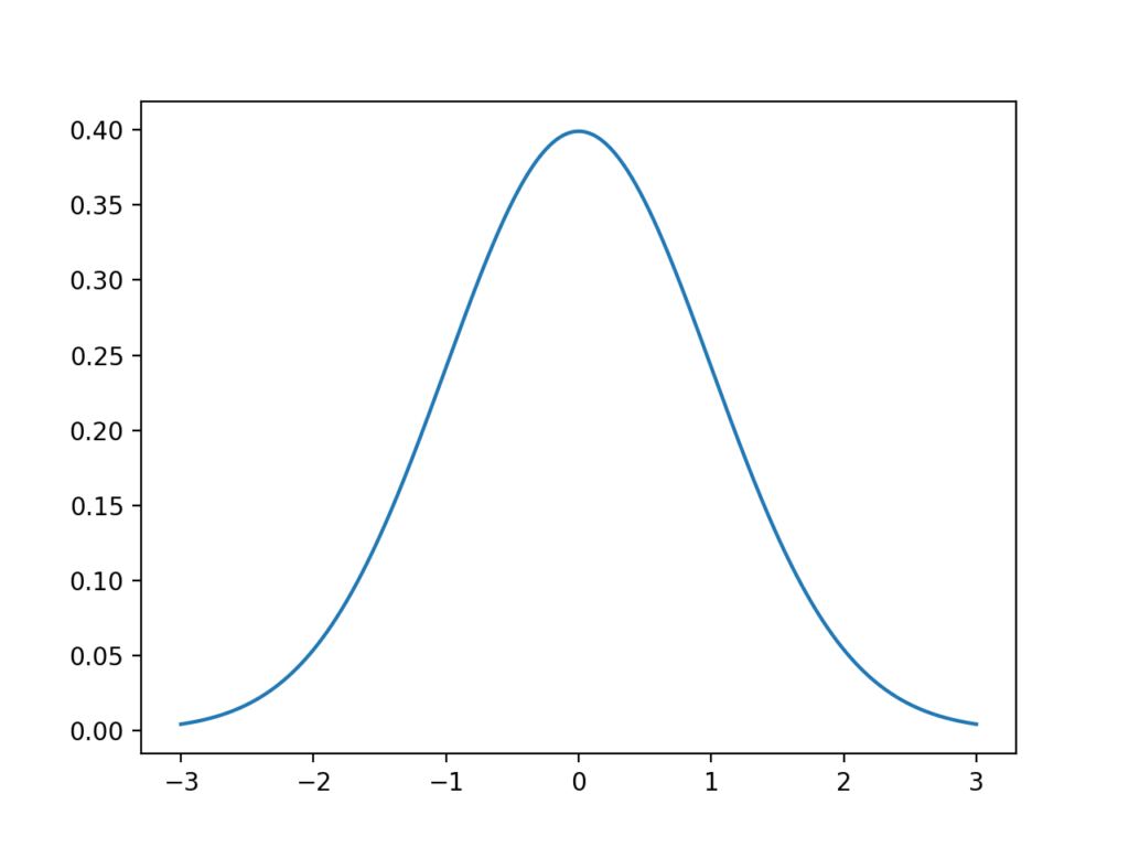Line Plot of Gaussian Distribution

It is helpful when data is Gaussian or when we assume a Gaussian distribution for calculating statistics. This is because the Gaussian distribution is very well understood. So much so that large parts of the field of statistics are dedicated to methods for this distribution.

Thankfully, many of the data we work with in machine learning often fits a Gaussian distribution, such as the input data we may use to fit a model, to the repeated evaluation of a model on different samples of training data.

Not all data is Gaussian, and it is sometimes important to make this discovery either by reviewing histogram plots of the data or using statistical tests to check. Some examples of observations that do not fit a Gaussian distribution include:

• People’s incomes.
• Population of cities.
• Sales of books.
  

Sample vs Population

We can think of data being generated by some unknown process.

The data that we collect is called a data sample, whereas all possible data that could be collected is called the population.

• Data Sample: A subset of observations from a group.
• Data Population: All possible observations from a group.
  

This is an important distinction because different statistical methods are used on samples vs populations, and in applied machine learning, we are often working with samples of data. If you read or use the word “population” when talking about data in machine learning, it very likely means sample when it comes to statistical methods.

Two examples of data samples that you will encounter in machine learning include:

• The train and test datasets.
• The performance scores for a model.
  

When using statistical methods, we often want to make claims about the population using only observations in the sample.

Two clear examples of this include:

• The training sample must be representative of the population of observations so that we can fit a useful model.
• The test sample must be representative of the population of observations so that we can develop an unbiased evaluation of the model skill.
  

Because we are working with samples and making claims about a population, it means that there is always some uncertainty, and it is important to understand and report this uncertainty.

Test Dataset

Before we explore some important summary statistics for data with a Gaussian distribution, let’s first generate a sample of data that we can work with.

We can use the randn() NumPy function to generate a sample of random numbers drawn from a Gaussian distribution.

There are two key parameters that define any Gaussian distribution; they are the mean and the standard deviation. We will go more into these parameters later as they are also key statistics to estimate when we have data drawn from an unknown Gaussian distribution.

The randn() function will generate a specified number of random numbers (e.g. 10,000) drawn from a Gaussian distribution with a mean of zero and a standard deviation of 1. We can then scale these numbers to a Gaussian of our choosing by rescaling the numbers.

This can be made consistent by adding the desired mean (e.g. 50) and multiplying the value by the standard deviation (5).

data = 5 * randn(10000) + 50

We can then plot the dataset using a histogram and look for the expected shape of the plotted data.

The complete example is listed below.

# generate a sample of random gaussians from numpy.random import seed from numpy.random import randn from matplotlib import pyplot # seed the random number generator seed(1) # generate univariate observations data = 5 * randn(10000) + 50 # histogram of generated data pyplot.hist(data) pyplot.show()

Running the example generates the dataset and plots it as a histogram.

We can almost see the Gaussian shape to the data, but it is blocky. This highlights an important point.

Sometimes, the data will not be a perfect Gaussian, but it will have a Gaussian-like distribution. It is almost Gaussian and maybe it would be more Gaussian if it was plotted in a different way, scaled in some way, or if more data was gathered.

Often, when working with Gaussian-like data, we can treat it as Gaussian and use all of the same statistical tools and get reliable results.

Histogram plot of Gaussian Dataset

In the case of this dataset, we do have enough data and the plot is blocky because the plotting function chooses an arbitrary sized bucket for splitting up the data. We can choose a different, more granular way to split up the data and better expose the underlying Gaussian distribution.

The updated example with the more refined plot is listed below.

# generate a sample of random gaussians from numpy.random import seed from numpy.random import randn from matplotlib import pyplot # seed the random number generator seed(1) # generate univariate observations data = 5 * randn(10000) + 50 # histogram of generated data pyplot.hist(data, bins=100) pyplot.show()

Running the example, we can see that choosing 100 splits of the data does a much better job of creating a plot that clearly shows the Gaussian distribution of the data.

The dataset was generated from a perfect Gaussian, but the numbers were randomly chosen and we only chose 10,000 observations for our sample. You can see, even with this controlled setup, there is obvious noise in the data sample.

This highlights another important point: that we should always expect some noise or limitation in our data sample. The data sample will always contain errors compared to the pure underlying distribution.

Histogram plot of Gaussian Dataset With More Bins

扫码加我 拉你入群

请注明：姓名-公司-职位

以便审核进群资格，未注明则拒绝

分享0 收藏0 回帖

关键词：introduction Calculating Statistics troduction statistic

Central Tendency

The central tendency of a distribution refers to the middle or typical value in the distribution. The most common or most likely value.

In the Gaussian distribution, the central tendency is called the mean, or more formally, the arithmetic mean, and is one of the two main parameters that defines any Gaussian distribution.

The mean of a sample is calculated as the sum of the observations divided by the total number of observations in the sample.

mean = sum(data) / length(data)

It is also written in a more compact form as:

mean = 1 / length(data) * sum(data)

We can calculate the mean of a sample by using the mean() NumPy function on an array.

result = mean(data)

The example below demonstrates this on the test dataset developed in the previous section.

# calculate the mean of a sample from numpy.random import seed from numpy.random import randn from numpy import mean # seed the random number generator seed(1) # generate univariate observations data = 5 * randn(10000) + 50 # calculate mean result = mean(data) print('Mean: %.3f' % result)

Running the example calculates and prints the mean of the sample.

This calculation of the arithmetic mean of the sample is an estimate of the parameter of the underlying Gaussian distribution of the population from which the sample was drawn. As an estimate, it will contain errors.

Because we know the underlying distribution has the true mean of 50, we can see that the estimate from a sample of 10,000 observations is reasonably accurate.

Mean: 50.049

The mean is easily influenced by outlier values, that is, rare values far from the mean. These may be legitimately rare observations on the edge of the distribution or errors.

Further, the mean may be misleading. Calculating a mean on another distribution, such as a uniform distribution or power distribution, may not make a lot of sense as although the value can be calculated, it will refer to a seemingly arbitrary expected value rather than the true central tendency of the distribution.

In the case of outliers or a non-Gaussian distribution, an alternate and commonly used central tendency to calculate is the median.

The median is calculated by first sorting all data and then locating the middle value in the sample. This is straightforward if there is an odd number of observations. If there is an even number of observations, the median is calculated as the average of the middle two observations.

We can calculate the median of a sample of an array by calling the median() NumPy function.

result = median(data)

The example below demonstrates this on the test dataset.

# calculate the median of a sample from numpy.random import seed from numpy.random import randn from numpy import median # seed the random number generator seed(1) # generate univariate observations data = 5 * randn(10000) + 50 # calculate median result = median(data) print('Median: %.3f' % result)

Running the example, we can see that median is calculated from the sample and printed.

The result is not too dissimilar from the mean because the sample has a Gaussian distribution. If the data had a different (non-Gaussian) distribution, the median may be very different from the mean and perhaps a better reflection of the central tendency of the underlying population.

Median: 50.042
Variance

The variance of a distribution refers to how much on average that observations vary or differ from the mean value.

It is useful to think of the variance as a measure of the spread of a distribution. A low variance will have values grouped around the mean (e.g. a narrow bell shape), whereas a high variance will have values spread out from the mean (e.g. a wide bell shape.)

We can demonstrate this with an example, by plotting idealized Gaussians with low and high variance. The complete example is listed below.

# generate and plot gaussians with different variance from numpy import arange from matplotlib import pyplot from scipy.stats import norm # x-axis for the plot x_axis = arange(-3, 3, 0.001) # plot low variance pyplot.plot(x_axis, norm.pdf(x_axis, 0, 0.5)) # plot high variance pyplot.plot(x_axis, norm.pdf(x_axis, 0, 1)) pyplot.show()

Running the example plots two idealized Gaussian distributions: the blue with a low variance grouped around the mean and the orange with a higher variance with more spread.

Line plot of Gaussian distributions with low and high variance

The variance of a data sample drawn from a Gaussian distribution is calculated as the average squared difference of each observation in the sample from the sample mean:

variance = 1 / (length(data) - 1) * sum(data - mean(data))^2

Where variance is often denoted as s^2 clearly showing the squared units of the measure. You may see the equation without the (- 1) from the number of observations, and this is the calculation of the variance for the population, not the sample.

We can calculate the variance of a data sample in NumPy using the var() function.

The example below demonstrates calculating variance on the test problem.

# calculate the variance of a sample from numpy.random import seed from numpy.random import randn from numpy import var # seed the random number generator seed(1) # generate univariate observations data = 5 * randn(10000) + 50 # calculate variance result = var(data) print('Variance: %.3f' % result)

Running the example calculates and prints the variance.

Variance: 24.939

It is hard to interpret the variance because the units are the squared units of the observations. We can return the units to the original units of the observations by taking the square root of the result.

For example, the square root of 24.939 is about 4.9.

Often, when the spread of a Gaussian distribution is summarized, it is described using the square root of the variance. This is called the standard deviation. The standard deviation, along with the mean, are the two key parameters required to specify any Gaussian distribution.

We can see that the value of 4.9 is very close to the value of 5 for the standard deviation specified when the samples were created for the test problem.

We can wrap the variance calculation in a square root to calculate the standard deviation directly.

standard deviation = sqrt(1 / (length(data) - 1) * sum(data - mean(data))^2)

Where the standard deviation is often written as s or as the Greek lowercase letter sigma.

The standard deviation can be calculated directly in NumPy for an array via the std() function.

The example below demonstrates the calculation of the standard deviation on the test problem.

# calculate the standard deviation of a sample from numpy.random import seed from numpy.random import randn from numpy import std # seed the random number generator seed(1) # generate univariate observations data = 5 * randn(10000) + 50 # calculate standard deviation result = std(data) print('Standard Deviation: %.3f' % result)

Running the example calculates and prints the standard deviation of the sample. The value matches the square root of the variance and is very close to 5.0, the value specified in the definition of the problem.

Standard Deviation: 4.994

Measures of variance can be calculated for non-Gaussian distributions, but generally require the distribution to be identified so that a specialized measure of variance specific to that distribution can be calculated.

支持一下

谢谢分享