Marginal effect estimation for predictors in logistic and probit models

是 否 +2 论坛币

k人 参与回答

经管之家送您一份

应届毕业生专属福利!

求职就业群

赵安豆老师微信：zhaoandou666

经管之家联合CDA

送您一个全额奖学金名额~ !

立即领取

感谢您参与论坛问题回答

经管之家送您两个论坛币！

+2 论坛币

The marginal effect of a predictor in a categorical response model estimates how much the probability of a response level changes as the predictor changes. For a continuous predictor, the marginal effect is defined as the partial derivative of the event probability with respect to the predictor of interest. For a binary categorical predictor, it is the change in event probability when the predictor is changed between its levels.

As a derivative, the marginal effect is the slope of a line drawn tangent to the fitted probability curve at the selected point. It is the instantaneous rate of change of the probability at that point. Note that the marginal effect depends on the predictor setting that corresponds to the selected point at which this tangent line is drawn, so the marginal effect of a variable is not constant. A measure of the overall effect of the predictor is the average of the marginal effects (AME). An alternative overall measure is marginal effect evaluated at the mean of all of the predictors (MEM). For small samples, the AME is considered the better measure.

Note that if the fitted probability curve is approximately linear (as it is near p=0.5) at the selected point, then the tangent line will closely approximate the fitted curve and the marginal effect will closely approximate the change in probability when changing the predictor by a fixed amount such as one unit. But in areas where the curve is nonlinear (near the smallest and largest values of p), the marginal effect might deviate substantially from the change over a fixed amount.

For a categorical predictor, the derivative is not strictly defined. In this case, the marginal effect is measured by the change in predicted probability between its levels.

For a binary logistic main-effects model, logit(p)=Σixiβi , the marginal effect of xi is equal to p(1–p)bi , where p is the event probability at the chosen setting of the predictors and bi is the parameter estimate for xi . The binary probit main-effects model is Φ-1(p)=Σixiβi , where Φ-1 is the inverse of the cumulative normal distribution function, or probit. The marginal effect of xi in the probit model is equal to φ(x'b)bi , where φ(x'b) is the density function of the standard normal distribution evaluated at x'b, x'b is the product of the row vector of chosen covariate values, x, and the column vector of parameter estimates, b, and bi is the parameter estimate for xi .

Marginal effects for continuous and categorical predictors in binary response models are available using the Margins macro. The Margins macro can also estimate and test predictive margins and marginal effects in other generalized linear models such as Poisson and gamma models and in Generalized Estimating Equations models. Additionally, point estimates of marginal effects for continuous predictors in binary or ordinal responses in main effects models are available in PROC QLIM in SAS/ETS® software by specifying the MARGINAL option in the OUTPUT statement.

Example: Binary logistic model

This example illustrates estimating marginal effects in a binary logistic model. In addition to the Margins macro and PROC QLIM, the partial derivative can be computed using results from the procedure used to fit the model. Note that many SAS® procedures can fit the binary logistic model as discussed in this note on the kinds of logistic models available in SAS. This example uses the cancer remission data presented in the example titled "Stepwise Logistic Regression and Predicted Values" in the PROC LOGISTIC documentation.

Marginal effects using the Margins macro

The following call of the Margins macro estimates the average marginal effect (AME) for the BLAST predictor. Note that the macro code must first be downloaded and submitted in your SAS session in order to make it available for use. The macro first fits a logistic model (the default when dist=binomial is specified) with response variable REMISS and predictors BLAST and SMEAR. The probability of REMISS=1 is chosen for modeling by roptions=event='1'. The macro then estimates the marginal effect of the continuous predictor specified in effect=. A confidence interval is requested with options=cl.

      %Margins(data     = Remiss,               response = remiss,                roptions = event='1',               model    = blast smear,               dist     = binomial,               effect   = blast,               options  = cl)

The average marginal effect of BLAST is estimated to be 0.315. A 95% large-sample confidence interval is also provided as well as a test that the marginal effect is zero. The macro can be run again to estimate the average marginal effect for SMEAR.

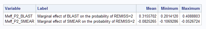
The average marginal effect for BLAST on REMISS=1 is 0.315 as found by the Margins macro above. The minimum and maximum marginal effects are also provided.

The same can be done for a probit model. In the Margins macro, specify link=probit. To fit the probit model in PROC QLIM, omit the D=LOGISTIC option from the previous code. The results (not shown) produce estimated marginal effects for BLAST similar to the values estimated under the logistic model.

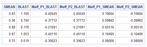
      %Margins(data     = Remiss,               response = remiss,                roptions = event='1',               model    = blast smear,               dist     = binomial,                link     = probit,               effect   = blast,               options  = cl)      proc qlim data=Remiss;        model remiss=blast smear / discrete;        output out=outqlim marginal;        run;      proc print data=outqlim (obs=5) noobs;        var smear blast meff:;        run;      proc means data=outqlim mean min max;        var Meff_P2:;        run;

扫码加我 拉你入群

请注明：姓名-公司-职位

以便审核进群资格，未注明则拒绝

分享0 收藏0 回帖

关键词：Predictors Estimation predictor Marginal logistic

Marginal effects using results from PROC LOGISTIC
As with PROC QLIM, the formulas used in the following are only appropriate for estimating point estimates of marginal effects for predictors not involved in interactions or higher-order effects in the model.

To compute the marginal effects using results from a model fit with PROC LOGISTIC, specify the OUTEST= option to save the parameter estimates in a data set. Also specify the P= option in the OUTPUT statement to save the predicted probabilities from the logistic model.

      proc logistic data=Remiss
           outest=logparms(rename=(blast=tblast smear=tsmear));
        model remiss(event="1")=blast smear;
        output out=outlog p=p;
        run;
Then use a DATA step to combine the OUTEST= and OUTPUT OUT= data sets and compute the marginal effects for each observation in the original data. Only the marginal effects for the response level representing the event of interest (REMISS=1) are computed below. The marginal effects for REMISS=0 could be similarly computed. The first five marginal effects are displayed by PROC PRINT and the average, minimum and maximum marginal effect are displayed by PROC MEANS.

      data outlog;
        if _n_=1 then set logparms;
        set outlog;
        MEffBlast = p*(1-p)*tblast;
        MEffSmear = p*(1-p)*tsmear;
        run;
      proc print data=outlog (obs=5) noobs;
        var smear blast MEff:;
        run;
      proc means data=outlog mean min max;
        var Meff:;
        run;
Notice that the estimated marginal effects match the previous results from the Margins macro and PROC QLIM.

The same can be done for a probit model. In the Margins macro, specify link=probit. To fit the probit model in PROC QLIM, omit the D=LOGISTIC option from the previous code. The results (not shown) produce estimated marginal effects for BLAST similar to the values estimated under the logistic model.

      %Margins(data     = Remiss,
               response = remiss,
               roptions = event='1',
               model    = blast smear,
               dist     = binomial,
               link     = probit,
               effect   = blast,
               options  = cl)
      proc qlim data=Remiss;
        model remiss=blast smear / discrete;
        output out=outqlim marginal;
        run;
      proc print data=outqlim (obs=5) noobs;
        var smear blast meff:;
        run;
      proc means data=outqlim mean min max;
        var Meff_P2:;
        run;
Marginal effects using results from PROC LOGISTIC
As with PROC QLIM, the formulas used in the following are only appropriate for estimating point estimates of marginal effects for predictors not involved in interactions or higher-order effects in the model.

To compute the marginal effects using results from a model fit with PROC LOGISTIC, specify the OUTEST= option to save the parameter estimates in a data set. Also specify the P= option in the OUTPUT statement to save the predicted probabilities from the logistic model.

      proc logistic data=Remiss
           outest=logparms(rename=(blast=tblast smear=tsmear));
        model remiss(event="1")=blast smear;
        output out=outlog p=p;
        run;
Then use a DATA step to combine the OUTEST= and OUTPUT OUT= data sets and compute the marginal effects for each observation in the original data. Only the marginal effects for the response level representing the event of interest (REMISS=1) are computed below. The marginal effects for REMISS=0 could be similarly computed. The first five marginal effects are displayed by PROC PRINT and the average, minimum and maximum marginal effect are displayed by PROC MEANS.

      data outlog;
        if _n_=1 then set logparms;
        set outlog;
        MEffBlast = p*(1-p)*tblast;
        MEffSmear = p*(1-p)*tsmear;
        run;
      proc print data=outlog (obs=5) noobs;
        var smear blast MEff:;
        run;
      proc means data=outlog mean min max;
        var Meff:;
        run;
Notice that the estimated marginal effects match the previous results from the Margins macro and PROC QLIM.



For the probit model, use the LINK=PROBIT option in PROC LOGISTIC (or use PROC PROBIT) to fit the model. Specify the XBETA= option in the OUTPUT statement to save the x'bvalues from the probit model. In a DATA step, combine the OUTEST= and OUTPUT OUT= data sets and use the PDF function to compute the marginal effects for the probit model.

      proc logistic data=Remiss
           outest=prbparms(rename=(blast=tblast smear=tsmear));
        model remiss(event="1")=blast smear / link=probit tech=newton;
        output out=outprb xbeta=xb;
        run;
      data outprb;
        if _n_=1 then set prbparms;
        set outprb;
        MEffBlast = pdf('NORMAL',xb)*tblast;
        MEffSmear = pdf('NORMAL',xb)*tsmear;
        run;
      proc print data=outprb (obs=5) noobs;
        var smear blast MEff:;
        run;
      proc means data=outprb mean min max;
        var Meff:;
        run;
Estimating the difference in probability at specific points
The effect of changing a predictor from one level to another can be directly computed by estimating pxi–pxj , the difference in event probabilities at levels i and j of the predictor. For a categorical predictor, xj is often an adjacent level (for ordinal predictors) or a reference level (for nominal predictors). For continuous predictors, it is common to look at the effect of a unit change in the predictor: px+1–px . But changes of more or less than one unit may be of interest.

The difference in probabilities can be estimated using the NLMeans macro after using the ESTIMATE statement in the modeling procedure to estimate the individual probabilities. For example, the following statements refit the model and the ESTIMATE statement estimates the probability of REMISS=1 at two settings one unit apart on the BLAST predictor and fixed at SMEAR=0.63. The ILINK option produces the estimate on the mean (probability) scale. The E option and the ODS OUTPUT statement and STORE statements are needed by the NLMeans macro. The macro uses the fitted model and the individual estimated probabilities to estimate and test the difference in probabilities. The EFFECTPLOT statement plots the estimated probability as a function of BLAST with SMEAR fixed at 0.63.

      proc logistic data=Remiss;
        model remiss(event="1")=blast smear;
        effectplot fit(x=blast) / at(smear=0.63) noobs nolimits;
        estimate 'Blast 1.5' intercept 1 blast 1.5 smear 0.63,
                 'Blast 0.5' intercept 1 blast 0.5 smear 0.63 / ilink e;
        ods output coef=coeffs;
        store log;
        run;
      %NLMeans(instore=log,
               coef=coeffs,
               link=logit,
               title=Blast 1.5-0.5 at Smear 0.63)
The plot shows how the predicted probability changes over the range of BLAST at SMEAR=0.63. The Mean column in the Estimates table produced by the ESTIMATE statement shows the individual probabilities as 0.25 and 0.63 at BLAST=0.5 and at 1.5. The difference, 0.38, displayed in the results from the NLMeans macro, is not significantly different from zero. A large-sample 95% confidence interval is also provided.



The same steps can be used for the probit model.

Marginal effects for higher-order models
As noted above, the marginal effect is the partial derivative of the event probability with respect to the variable of interest, xi:



For the case of simple main-effects models as discussed above, logit(p)=Σixiβi , the final partial derivative is just βi yielding p(1-p)βi as the marginal effect of xi as before. For a higher-order model, such as a model involving xi in an interaction or quadratic effect, the marginal effect is slightly more complex. Consider the cancer remission data and a model that includes the main effects of BLAST and SMEAR as well as their interaction:

logit(p) = β0 + βsSMEAR + βbBLAST + βsbSMEAR·BLAST

For this model, the partial derivative of x'β with respect to SMEAR is βs+βsbBLAST, so the marginal effect for SMEAR is p(1-p)(βs+βsbBLAST). Similarly for BLAST.

The average marginal effect for BLAST in the above model can be obtained using this call of the Margins macro.

      %Margins(data     = Remiss,
               response = remiss,
               roptions = event='1',
               model    = blast|smear,
               dist     = binomial,
               effect   = blast,
               options  = cl)
For this model with interaction, the average marginal effect of BLAST is estimated to be 0.373 and is significantly different from zero (p=0.0045).



Marginal effects for ordinal logistic models
Suppose the possible response values are ordered with levels i=1, 2, ... , k. Under the ordinal logistic model (proportional odds model), the probability of response level i is the difference in the cumulative probabilities at level i and level i-1.

pi = F(αi+x'β) - F(αi-1+x'β) ,

where αi is the ith intercept, β contains all non-intercept parameters, and F(x) is the logistic cumulative distribution function F(x)=exp(x)/(1+exp(x)). Then the marginal effect of the jthpredictor, xj, on pi is



For a model containing only main-effects,  = βj as in the binary logistic model discussed above. For more complex models, replace  with the resulting function.

The ordinal model can be fit in many procedures including LOGISTIC, PROBIT, GENMOD, GLIMMIX, QLIM, and NLMIXED. However, only PROC QLIM provides an option to compute marginal effect estimates. As for the binary response model, it should only be used to obtain marginal effect estimates for predictors not involved in interactions or higher-order effects in the model.

The following example uses the data from the example titled "Multilevel Response" in the PROC PROBIT documentation. The response is the severity of symptoms with ordered levels: none, mild, severe. These statements create the data set with a numerically coded response variable, Y, with levels 1, 2, and 3 corresponding to increasing severity of the symptoms.

      data multi;
        input Prep $ Dose Symptoms $ N;
        if symptoms='None' then y=1;
        else if symptoms='Mild' then y=2;
        else y=3;
        LDose=log10(Dose);
        datalines;
      stand     10      None       33
      stand     10      Mild        7
      stand     10      Severe     10
      stand     20      None       17
      stand     20      Mild       13
      stand     20      Severe     17
      stand     30      None       14
      stand     30      Mild        3
      stand     30      Severe     28
      stand     40      None        9
      stand     40      Mild        8
      stand     40      Severe     32
      test      10      None       44
      test      10      Mild        6
      test      10      Severe      0
      test      20      None       32
      test      20      Mild       10
      test      20      Severe     12
      test      30      None       23
      test      30      Mild        7
      test      30      Severe     21
      test      40      None       16
      test      40      Mild        6
      test      40      Severe     19
      ;
These statements fit the ordinal logistic model and display the marginal effect estimates. The ordinal probit model can be fit using the DISCRETE(DIST=NORMAL) option. PROC QLIM models the probabilities of higher response levels and cumulates the probabilities over the lower response levels.

      proc qlim data=multi;
        freq N;
        model y=LDose / discrete(dist=logit);
        output out=outqlim marginal;
        run;
      proc print data=outqlim noobs;
        where prep='stand';
        var y symptoms ldose meff:;
        run;
Notice that marginal effect estimates are provided for each response level of the predictor.

Marginal effects for nominal multinomial logistic models
Suppose the possible response values are unordered with levels i=1, 2, ... , k. Under the generalized logit model commonly used for nominal responses, the probability of response level i is

pi = exp(x'βi)/Σj(exp(x'βj))

Then the marginal effect of the jth predictor, xj, on pi is



For a model containing only main-effects,  = βij and  = βkj. For more complex models, replace these partial derivatives with the resulting functions.

The generalized logit model can be fit by the LOGISTIC, GLIMMIX, CATMOD, and NLMIXED procedures. Marginal effects are not directly available, but can be computed using the parameter estimates and individual predicted probabilities from any of these procedures.

The following example uses the remote-sensing data presented in the example titled "Scoring Data Sets" in the LOGISTIC documentation. The response is the type of crop with five possible levels. X1 is one of four variables used to predict the type of crop. The following statements fit a generalized logit model with X1 as predictor and saves the parameter estimates and individual predicted probabilities to data sets. Marginal effects are computed using the above formula for each of the crops using the values of X1 in each of the observations. Note that four generalized logits can be defined on the five crop types. Consequently, the parameter for the last crop type (Sugarbeets) is constrained to zero. The EFFECTPLOT statement produces a plot of the predicted probabilities for the individual response levels.

      proc logistic data=Crops
        outest=logparms;
        model crop = x1 / link=glogit;
        effectplot fit(x=x1) / noobs nolimits;
        output out=preds predprobs=individual;
        run;
      data margeff;
        if _n_=1 then set logparms;
        set preds;
        SumBetaPred=x1_clover*IP_Clover + x1_corn*IP_Corn +
                    x1_cotton*IP_Cotton + x1_soybeans*IP_Soybeans;
        MEClover    =IP_Clover*(x1_clover-SumBetaPred);
        MECorn      =IP_Corn*(x1_corn-SumBetaPred);
        MECotton    =IP_Cotton*(x1_cotton-SumBetaPred);
        MESoybeans  =IP_Soybeans*(x1_soybeans-SumBetaPred);
        MESugarbeets=IP_Sugarbeets*(-SumBetaPred);
        run;
      proc sort nodupkey;
        by x1;
        run;
      proc print;
        id x1;
        var ME:;
        run;
The values of the marginal effects reflect the slopes of lines tangent to each of the crop curves at each X1 setting. For instance, lines tangent to the Soybeans curve have positive slopes up to about 19, then become negative after 20, and essentially zero beyond 50.

yunnandlg 发表于 2019-10-11 16:32
The marginal effect of a predictor in a categorical response model estimates how much the probabilit ...

You believe in fate?
你相信命运吗？

Make some actual use of your life.
用你的生命去做些真正有意义的事吧！

摔倒是站起来的地方，坚强是伤口的结痂，经历是过去坎坷的成长。成熟在逆境，醒悟在绝境。在逆境中抓住背后的机遇，在绝境中创造奇迹。受苦，只是履行命运的一种方式，人生的一切都要由自己去承担。张扬生命的每次精彩，回味人生的每次困顿，沿着自己喜欢的方向慢慢摸索前行，在生命的曲折中自有坚持。

Living like a lusty flower.
像绽放的鲜花一般生活吧！

Note that the macro code must first be downloaded and submitted in your SAS session in order to make it available for use.？？？？请问怎么下载宏代码啊

请问怎么下载宏代码啊