TPOT: A Python Tool for Automating Data Science

是 否 +2 论坛币

k人 参与回答

经管之家送您一份

应届毕业生专属福利!

求职就业群

赵安豆老师微信：zhaoandou666

经管之家联合CDA

送您一个全额奖学金名额~ !

立即领取

感谢您参与论坛问题回答

经管之家送您两个论坛币！

+2 论坛币

Machine learning is often touted as:

A field of study that gives computers the ability to learn without being explicitly programmed.

Despite this common claim, anyone who has worked in the field knows that designing effective machine learning systems is a tedious endeavor, and typically requires considerable experience with machine learning algorithms, expert knowledge of the problem domain, and brute force search to accomplish. Thus, contrary to what machine learning enthusiasts would have us believe, machine learning still requires a considerable amount of explicit programming.

In this article, we’re going to go over three aspects of machine learning pipeline design that tend to be tedious but nonetheless important. After that, we’re going to step through a demo for a tool that intelligently automates the process of machine learning pipeline design, so we can spend our time working on the more interesting aspects of data science.

Let’s get started.

Model hyperparameter tuning is important

One of the most tedious parts of machine learning is model hyperparameter tuning.

Support vector machines require us to select the ideal kernel, the kernel’s parameters, and the penalty parameter C. Artificial neural networks require us to tune the number of hidden layers, number of hidden nodes, and many more hyperparameters. Even random forests require us to tune the number of trees in the ensemble at a minimum.

All of these hyperparameters can have significant impacts on how well the model performs. For example, on the MNIST handwritten digit data set:

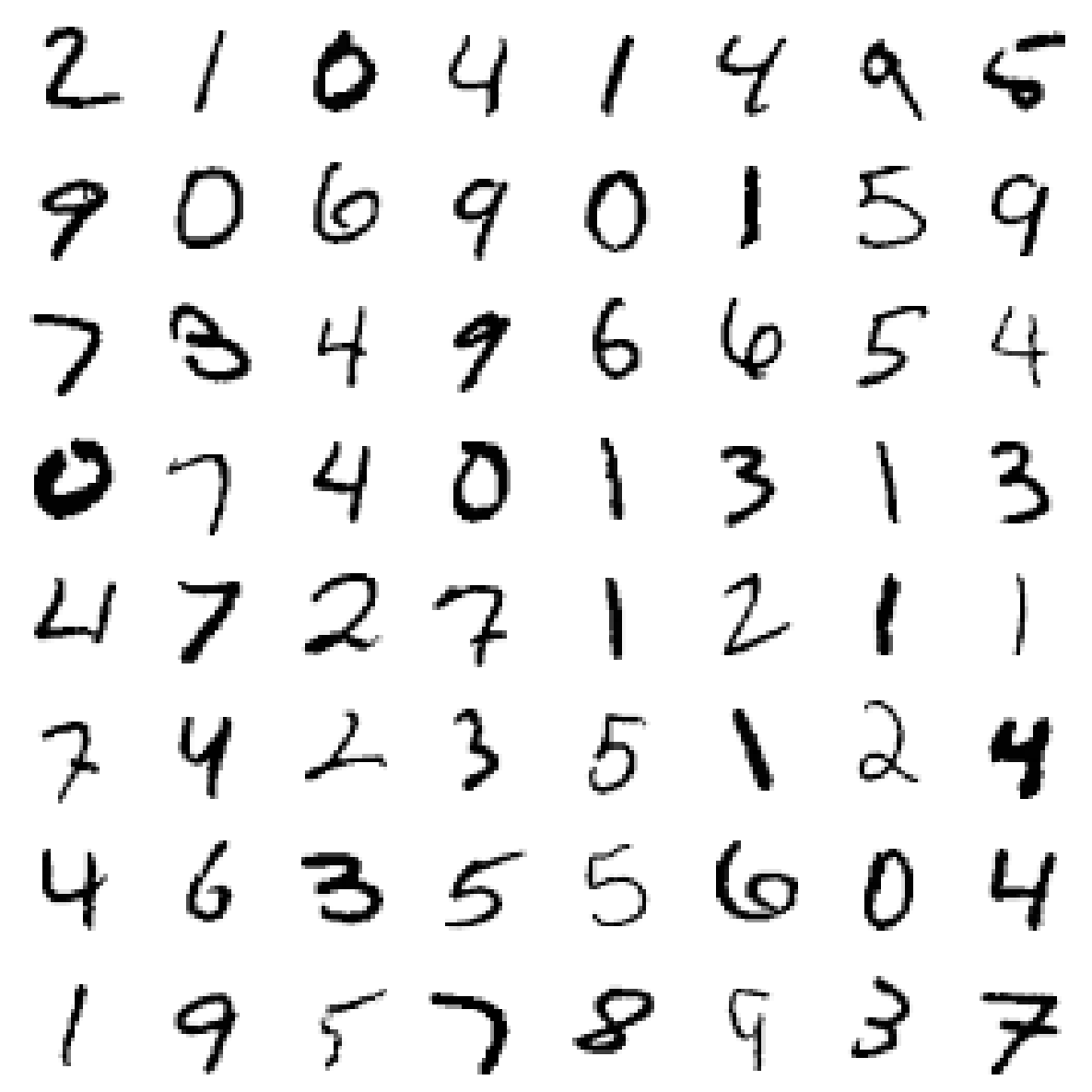
If we fit a random forest classifier with only 10 trees (scikit-learn’s default):

import pandas as pd  import numpy as np  from sklearn.ensemble import RandomForestClassifier  from sklearn.cross_validation import cross_val_score  mnist_data = pd.read_csv('https://raw.githubusercontent.com/rhiever/Data-Analysis-and-Machine-Learning-Projects/master/tpot-demo/mnist.csv.gz', sep='\t', compression='gzip')  cv_scores = cross_val_score(RandomForestClassifier(n_estimators=10, n_jobs=-1),                              X=mnist_data.drop('class', axis=1).values,                              y=mnist_data.loc[:, 'class'.values,                              cv=10)  print(cv_scores)  [ 0.93461813  0.96287836  0.94688749  0.94072275  0.95114286  0.94570653    0.94884253  0.94311848  0.93825043  0.95668954  print(np.mean(cv_scores))  0.946885709001

The random forest achieves an average of 94.7% cross-validation accuracy on MNIST. However, what if we tuned that hyperparameter a little bit and provided the random forest with 100 trees instead?

cv_scores = cross_val_score(RandomForestClassifier(n_estimators=100, n_jobs=-1),                              X=mnist_data.drop('class', axis=1).values,                              y=mnist_data.loc[:, 'class'.values,                              cv=10)  print(cv_scores)  [ 0.96259814  0.97829812  0.9684466   0.96700471  0.966       0.96399486    0.97113461  0.96755752  0.96397942  0.97684391  print(np.mean(cv_scores))  0.968585789367

With such a minor change, we improved the random forest’s average cross-validation accuracy from 94.7% to 96.9%. This small improvement in accuracy can translate into millions of additional digits classified correctly if we’re applying this model on the scale of, say, processing addresses for the U.S. Postal Service.

Never use the defaults for your model. Hyperparameter tuning is vitally important for every machine learning project.

Model selection is important

We all love to think that our favorite model will perform well on every machine learning problem, but different models are better suited for different tasks.

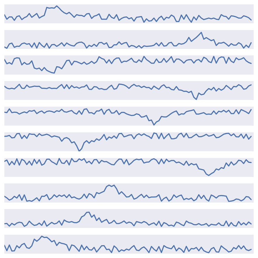
For example, if we’re working on a signal processing problem where we need to classify whether there’s a “hill” or “valley” in the time series:

And we apply a “tuned” random forest to the problem:

import pandas as pd  import numpy as np  from sklearn.ensemble import RandomForestClassifier  from sklearn.linear_model import LogisticRegression  from sklearn.cross_validation import cross_val_score    hill_valley_data = pd.read_csv('https://raw.githubusercontent.com/rhiever/Data-Analysis-and-Machine-Learning-Projects/master/tpot-demo/Hill_Valley_without_noise.csv.gz', sep='\t', compression='gzip')    cv_scores = cross_val_score(RandomForestClassifier(n_estimators=100, n_jobs=-1),                              X=hill_valley_data.drop('class', axis=1).values,                              y=hill_valley_data.loc[:, 'class'.values,                              cv=10)    print(cv_scores)    [ 0.64754098  0.64754098  0.57024793  0.61983471  0.62809917  0.61983471    0.70247934  0.59504132  0.49586777  0.65289256    print(np.mean(cv_scores))    0.617937948787

Then we’re going to find that the random forest isn’t well-suited for signal processing tasks like this one when it achieves a disappointing average of 61.8% cross-validation accuracy.

What if we tried a different model, for example a logistic regression?

cv_scores = cross_val_score(LogisticRegression(),                              X=hill_valley_data.drop('class', axis=1).values,                              y=hill_valley_data.loc[:, 'class'.values,                              cv=10)    print(cv_scores)    [ 1.          1.          1.          0.99173554  1.          0.98347107    1.          0.99173554  1.          1.            print(np.mean(cv_scores))    0.996694214876

We’ll find that a logistic regression is well-suited for this signal processing task—in fact, it easily achieves near-100% cross-validation accuracy without any hyperparameter tuning at all.

Always try out many different machine learning models for every machine learning task that you work on. Trying out—and tuning—different machine learning models is another tedious yet vitally important step of machine learning pipeline design.

扫码加我 拉你入群

请注明：姓名-公司-职位

以便审核进群资格，未注明则拒绝

分享0 收藏0 回帖

关键词：Data Science Science python MATIN Auto experience computers effective knowledge learning

Feature preprocessing is important

As we’ve seen in the previous two examples, machine learning model performance is also affected by how the features are represented. Feature preprocessing is a step in machine learning pipelines where we reshape the features in a manner that makes the data set easier for models to classify.

For example, if we’re working on a harder version of the “hill” vs. “valley” signal processing problem with noise:

And we apply a “tuned” random forest to the problem:

import pandas as pd  import numpy as np  from sklearn.ensemble import RandomForestClassifier  from sklearn.decomposition import PCA  from sklearn.pipeline import make_pipeline  from sklearn.cross_validation import cross_val_score    hill_valley_noisy_data = pd.read_csv('https://raw.githubusercontent.com/rhiever/Data-Analysis-and-Machine-Learning-Projects/master/tpot-demo/Hill_Valley_with_noise.csv.gz', sep='\t', compression='gzip')    cv_scores = cross_val_score(RandomForestClassifier(n_estimators=100, n_jobs=-1),                              X=hill_valley_noisy_data.drop('class', axis=1).values,                              y=hill_valley_noisy_data.loc[:, 'class'.values,                              cv=10)    print(cv_scores)    [ 0.52459016  0.51639344  0.57377049  0.6147541   0.6557377   0.56557377    0.575       0.575       0.60833333  0.575         print(np.mean(cv_scores))    0.578415300546

We’ll again find that the “tuned” random forest averages a disappointing 57.8% cross-validation accuracy.

However, if we preprocess the features—denoising them via Principal Component Analysis (PCA), for example:

cv_scores = cross_val_score(make_pipeline(PCA(n_components=10),                                            RandomForestClassifier(n_estimators=100,                                                                   n_jobs=-1)),                              X=hill_valley_noisy_data.drop('class', axis=1).values,                              y=hill_valley_noisy_data.loc[:, 'class'.values,                              cv=10)    print(cv_scores)    [ 0.96721311  0.98360656  0.8852459   0.96721311  0.95081967  0.93442623    0.91666667  0.89166667  0.94166667  0.95833333    print(np.mean(cv_scores))    0.93968579235

We’ll find that the random forest now achieves an average of 94% cross-validation accuracy by applying a simple feature preprocessing step.

Always explore numerous feature representations for your data. Machines learn differently from humans, and a feature representation that makes sense to us may not make sense to the machine.

Automating data science with TPOT

To summarize what we’ve learned so far about effective machine learning system design, we should:

• Always tune the hyperparameters for our models
• Always try out many different models
• Always explore numerous feature representations for our data
  

This is why it can be so tedious to design effective machine learning systems. This is also why my collaborators and I created TPOT, an open source Python tool that intelligently automates the entire process.

If your data set is compatible with scikit-learn, then TPOT will automatically optimize a series of feature preprocessors and models that maximize the cross-validation accuracy on the data set. For example, if we want TPOT to solve the noisy “hill” vs. “valley” classification problem:

(Before running the code below, make sure to install TPOT first.)

import pandas as pd  from sklearn.cross_validation import train_test_split  from tpot import TPOT    hill_valley_noisy_data = pd.read_csv('https://raw.githubusercontent.com/rhiever/Data-Analysis-and-Machine-Learning-Projects/master/tpot-demo/Hill_Valley_with_noise.csv.gz', sep='\t', compression='gzip')    X = hill_valley_noisy_data.drop('class', axis=1).values  y = hill_valley_noisy_data.loc[:, 'class'.values    X_train, X_test, y_train, y_test = train_test_split(X, y,                                                      train_size=0.75,                                                      test_size=0.25)    my_tpot = TPOT(generations=10)  my_tpot.fit(X_train, y_train)    print(my_tpot.score(X_test, y_test))    0.960352039038

Depending on the machine you’re running it on, 10 TPOT generations should take about 5 minutes to complete. During this time, you’re free to browse Hacker News, refill your cup of coffee, or admire the beautiful weather outside. In the meantime, TPOT will handle all of the work for you.

After 5 minutes of optimization, TPOT will discover a pipeline that achieves 96% cross-validation accuracy on the noisy “hill” vs. “valley” problem—better than the hand-designed pipeline we created above!

If we want to see what pipeline TPOT created, TPOT can export the corresponding scikit-learn code for us with the export() command:

my_tpot.export('exported_pipeline.py')

which will look something like:

import pandas as pd  from sklearn.cross_validation import train_test_split  from sklearn.linear_model import LogisticRegression    # NOTE: Make sure that the class is labeled 'class' in the data file  tpot_data = pd.read_csv('https://raw.githubusercontent.com/rhiever/Data-Analysis-and-Machine-Learning-Projects/master/tpot-demo/Hill_Valley_with_noise.csv.gz', sep='\t', compression='gzip')    training_indices, testing_indices = train_test_split(tpot_data.index,                                                       stratify=tpot_data['class'.values,                                                       train_size=0.75,                                                       test_size=0.25)    result1 = tpot_data.copy()    # Perform classification with a logistic regression classifier  lrc1 = LogisticRegression(C=0.0001)  lrc1.fit(result1.loc[training_indices.drop('class', axis=1).values,           result1.loc[training_indices, 'class'.values)  result1['lrc1-classification' = lrc1.predict(result1.drop('class', axis=1).values)

and shows us that a tuned logistic regression is probably the best model for this problem

oliyiyi 发表于 2016-8-19 10:01
Machine learning is often touted as:A field of study that gives computers the ability to learn witho ...

谢谢楼主的分享