[貝葉斯專著]Bayesian Item Response Modeling(using WinBUGS)

相似文件 换一批

是 否 +2 论坛币

k人 参与回答

经管之家送您一份

应届毕业生专属福利!

求职就业群

赵安豆老师微信：zhaoandou666

经管之家联合CDA

送您一个全额奖学金名额~ !

立即领取

感谢您参与论坛问题回答

经管之家送您两个论坛币！

+2 论坛币

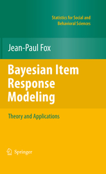
Bayesian Item Response Modeling:Theory and Applications

Fox, Jean-Paul

2010, XIV, 313p.

• Serves as a handbook for measurement specialists and a textbook for students on the Bayesian approach to modern test theory.
• Acts as a guide to the authors’ computer software implementations that will be made available via a website.
• Includes software implementations available in S-Plus and R, with new functions built on Fortran code linked to the S-plus and R environments, for time efficiency.
  
  

This book presents a thorough treatment and unified coverage of Bayesian item response modeling with applications in a variety of disciplines, including education, medicine, psychology, and sociology. Breakthroughs in computing technology have made the Bayesian approach particularly useful for many response modeling problems. Free from computational constraints, realistic and state-of-the-art latent variable response models are considered for complex assessment and survey data to solve real-world problems. The Bayesian framework described provides a unified approach for modeling and inference, dealing with (nondata) prior information and information across multiple data sources. The book discusses methods for analyzing item response data and the complex relationships commonly associated with human response behavior and features

• Self-contained introduction to Bayesian item response modeling and a coverage of extending standard models to handle complex assessment data
• A thorough overview of Bayesian estimation and testing methods for item response models, where MCMC methods are emphasized
• Numerous examples that cover a wide range of application areas, including education, medicine, psychology, and sociology
• Datasets and software (S+, R, and WinBUGS code) of the models and methods presented in the book are available on www.jean-paulfox.com Bayesian Item Response Modeling is an excellent book for research professionals, including applied statisticians, psychometricians, and social scientists who analyze item response data from a Bayesian perspective. It is a guide to the growing area of Bayesian response modeling for researchers and graduate students, and will also serve them as a good reference. Jean-Paul Fox is Associate Professor of Measurement and Data Analysis, University of Twente, The Netherlands. His main research activities are in several areas of Bayesian response modeling. Dr. Fox has published numerous articles in the areas of Bayesian item response analysis, statistical methods for analyzing multivariate categorical response data, and nonlinear mixed effects models.
• 
  

本帖隐藏的内容

Bayesian IRT.pdf (4.14 MB, 需要: 25 个论坛币)

2014-7-3 05:41:50 上传

Bayesian Item Response Modeling
需要: 25 个论坛币  [购买]

http://www.jean-paulfox.com/index.php?option=com_content&view=category&id=5&layout=blog&Itemid=3

扫码加我 拉你入群

请注明：姓名-公司-职位

以便审核进群资格，未注明则拒绝

分享0 收藏10 回帖

关键词：Modeling response Bayesian winbugs WINBUG available software computer linked

WinBUGS Programs/Code for various applications

WinBUGS-Code 'Bayesian Item Response Modeling'Chapter 1: Modeling Examinees' Test Results (Data and Code): (Test Data) and (Two-Parameter Item response Model) Chapter 2: Mathematics Placement Test (Data (Ordinal Data Modeling, Johnson and Albert, 1999), Code): (Placement Test Data (WinBUGS)) (Hierarchical Item Prior (WinBUGS)) (Independent Item Prior (WinBUGS)) (Three-Parameter Simple Prior (WinBUGS)) Chapter 4: TIMMS (2007) Dutch Sixth-Graders Math Achievement (TIMMS 2007, 6th Graders' Math Achievement) (TIMMS 2007, 6th Graders' Math Achievement Data (include gender)) (TIMMS 2007: Hierarchical Item Prior (WinBUGS)) (TIMMS 2007: Linear Latent Structure (WinBUGS)) ESS: Measuring Political Interest (ESS Netherlands: Items Measuring Political Interest) (ESS: Graded Item Response Model (WinBUGS)) Chapter 5: Dutch Primary School Mathematics Test (Dutch Primary School Leaving Test) Chapter 8: Rule-Based Item Test (Rule-Based Items (Exercise 8.1)) (Rule-Based Items (Exercise 8.3)) (One-Parameter Response-Time Model and Item Response (WinBUGS)) (One-Parameter Response-Time Model and Item Responses (WinBUGS))

Two-parameter Item Response Model using Splus

1. #  Estimate Two-Parameter Normal Ogive Model. J.-P. Fox, University of Twente, Augustus 2010.
   
2. 
   
3. ## K:: number of items
   
4. ## N:: number persons
   
5. 
   
6. ## DrawZ. Data Augmentation Z: Normal Ogive Model
   
7. ##        DrawTheta. Draw values latent variable theta
   
8. ## DrawBeta. Draw values difficulty parameter beta0
   
9. ## DrawAlpha. Draw values discrimination parameter alpha0
   
10. 
    
11. DrawZ         <- function(alpha0,beta0,theta0,Y){
    
12.         N                 <- nrow(Y)
    
13.         K                 <- ncol(Y)
    
14.         eta                <- t(matrix(alpha0, ncol = N, nrow= K)) * matrix(theta0,ncol=K,nrow=N) - t(matrix(beta0, ncol = N, nrow = K))
    
15.         BB                <- matrix(pnorm(-eta),ncol = K, nrow = N)
    
16.         u                <- matrix(runif(N*K), ncol = K, nrow = N)
    
17.         tt                <- matrix( ( BB*(1-Y) + (1-BB)*Y )*u + BB*Y, ncol = K, nrow = N)
    
18.         Z                <- matrix(qnorm(tt),ncol = K, nrow = N) + matrix(eta,ncol = K, nrow = N)
    
19.   return(Z)
    
20. }
    
21. 
    
22. DrawTheta <- function(alpha0,beta0,Z) {
    
23. #prior theta N(0,1)
    
24.         N                <- nrow(Z)
    
25.         K                 <- ncol(Z)
    
26.         pvar                <- (sum(alpha0^2)+1)
    
27.         thetahat        <- (((Z + t(matrix(beta0,ncol= N, nrow = K))) %*% matrix(alpha0,ncol = 1,nrow = K)))
    
28.         mu                <- thetahat/pvar
    
29.         theta                <- rnorm(N,mean=mu,sd=sqrt(1/pvar))
    
30.         theta                <- (theta - mean(theta))#/sqrt(var(theta))
    
31. return(theta)
    
32. }
    
33. 
    
34. 
    
35. DrawBeta <- function(alpha0,theta0,Z) {
    
36. # diffuse prior       
    
37.         N                <- nrow(Z)
    
38.         K                <- ncol(Z)
    
39.         Zp                <- t(matrix(alpha0,nrow= K,ncol = N)) * matrix(theta0,ncol=K,nrow=N) - matrix(Z,ncol=K,nrow=N)
    
40.         mu                <- apply(Zp,2,sum)/N
    
41.         beta          <- matrix(rnorm(K,mean=mu,sd=sqrt(1/N)),ncol=1,nrow=K)
    
42. return(beta)
    
43. }
    
44. 
    
45. DrawAlpha <- function(beta0,theta0,Z){
    
46. # diffuse prior
    
47.         N                <- nrow(Z)
    
48.         K                <- ncol(Z)
    
49.         Zp                <- (matrix(Z,ncol=K,nrow=N) + t(matrix(beta0,nrow=K,ncol=N))) * matrix(theta0,nrow=N,ncol=K)
    
50.         mu                 <- apply(Zp,2,sum)/sum(theta0^2)
    
51.         alpha         <- matrix(rnorm(K,mean=mu,sd=sqrt(1/sum(theta0^2))),ncol=1,nrow=K)
    
52. return(alpha)
    
53. }
    
54. 
    
55. 
    
56. TWOPNO <- function(Y,XG)
    
57. {
    
58.         N                 <- nrow(Y)
    
59.         K                 <- ncol(Y)
    
60. 
    
61. #Initialise
    
62.         alpha0         <- matrix(1,ncol = 1, nrow = 1)
    
63.         beta0                 <- matrix(0,ncol=1,nrow=1)
    
64.         theta0         <- matrix(rnorm(N),ncol=1,nrow=N)
    
65.         EAPtheta         <- matrix(0,ncol=1,nrow=N)
    
66.         SQtheta         <- matrix(0,ncol=1,nrow=N)
    
67.         Malpha         <- matrix(0,ncol=K,nrow=XG)
    
68.         Mbeta                 <- matrix(0,ncol=K,nrow=XG)
    
69. 
    
70. for(ii in 1:XG){
    
71. 
    
72.         Z                                        <- DrawZ(alpha0,beta0,theta0,Y)
    
73.         theta0                                <- DrawTheta(alpha0,beta0,Z)
    
74.         beta0                                <- DrawBeta(alpha0,theta0,Z)
    
75.         alpha0                         <- DrawAlpha(beta0,theta0,Z)       
    
76.         EAPtheta                         <- ((ii - 1)*EAPtheta + theta0)/ii
    
77.         SQtheta                        <- ((ii - 1)*SQtheta + theta0^2)/ii
    
78.         Malpha[ii,1:K]        <- alpha0[1:K]
    
79.         Mbeta[ii,1:K]         <- beta0[1:K]
    
80. }       
    
81.        
    
82.         return(list(Malpha,Mbeta,EAPtheta,SQtheta))
    
83. }
    
84. 
    
85. 
    
86. N        <- 1000
    
87. K        <- 20
    
88. sim                <-        sim2PNO(N,K)
    
89. Y                <-         matrix(sim[[1]],ncol=K,nrow=N)
    
90. theta        <-         matrix(sim[[2]],ncol=1,nrow=N)
    
91. alpha        <-         matrix(sim[[3]],ncol=1,nrow=K)
    
92. beta         <-         matrix(sim[[4]],ncol=1,nrow=K)
    
93. 
    
94. out <- TWOPNO(Y,XG=1000)
    
95. Malpha <- matrix(out[[1]],ncol=K)
    
96. Mbeta <- matrix(out[[2]],ncol =K)
    
97. EAPtheta <- out[[3]]
    
98. SDtheta <- sqrt(out[[4]] - out[[3]]^2) ### estimate standard deviation theta
    
99. 
    
100. plot(theta[1:N],EAPtheta[1:N])
     
101. abline(0,1)
     
102. 
     
103. ### Use estMLIRT program
     
104. S <- c(0,0,0,0)
     
105. out2 <- estMLIRT(Y, S, nll=N, XG=1000)
     
106. MLIRTout(500,out2)

复制代码

1. #  Estimate Rasch Model. J.-P. Fox, University of Twente, Augustus 2010.
   
2. 
   
3. ## K:: number of items
   
4. ## N:: number persons
   
5. 
   
6. ## DrawZ. Data Augmentation Z: Normal Ogive Model
   
7. ##        DrawTheta. Draw values latent variable theta
   
8. ## DrawBeta. Draw values difficulty parameter
   
9. ## IRT. Main Program.
   
10. 
    
11. DrawZ         <- function(beta0,theta0,Y){
    
12.         N                 <- nrow(Y)
    
13.         K                 <- ncol(Y)
    
14.         eta                <- matrix(theta0,ncol=K,nrow=N) - t(matrix(beta0, ncol = N, nrow = K))
    
15.         BB                <- matrix(pnorm(-eta),ncol = K, nrow = N)
    
16.         u                <- matrix(runif(N*K), ncol = K, nrow = N)
    
17.         tt                <- matrix( ( BB*(1-Y) + (1-BB)*Y )*u + BB*Y, ncol = K, nrow = N)
    
18.         Z                <- matrix(qnorm(tt),ncol = K, nrow = N) + matrix(eta,ncol = K, nrow = N)
    
19.   return(Z)
    
20. }
    
21. 
    
22. DrawTheta <- function(beta0,Z) {
    
23. #prior theta N(0,1)
    
24.         N                <- nrow(Z)
    
25.         K                 <- ncol(Z)
    
26.         pvar                <- K + 1
    
27.         thetahat        <- ((Z + t(matrix(beta0,ncol= N, nrow = K))) %*% matrix(1,ncol = 1,nrow = K))
    
28.         mu                <- thetahat/pvar
    
29.         theta        <- matrix(rnorm(N,mean=mu,sd=sqrt(1/pvar)),ncol=1,nrow=N)
    
30.   return(theta)
    
31. }
    
32. 
    
33. 
    
34. DrawBeta <- function(theta0,Z) {
    
35. # diffuse prior       
    
36.         N        <- nrow(Z)
    
37.         K        <- ncol(Z)
    
38.         Zp        <- matrix(theta0,ncol=K,nrow=N) - matrix(Z,ncol=K,nrow=N)
    
39.         mu        <- apply(Zp,2,sum)/N
    
40.         beta <- matrix(rnorm(K,mean=mu,sd=sqrt(1/N)),ncol=1,nrow=K)
    
41. return(beta)
    
42. }
    
43. 
    
44. 
    
45. IRT <- function(Y,XG)
    
46. {
    
47. 
    
48. ## Initialise
    
49. 
    
50. N        <- nrow(Y)
    
51. K        <- ncol(Y)
    
52. 
    
53. beta0 <- matrix(0,ncol=1,nrow=1)
    
54. theta0 <- matrix(rnorm(N),ncol=1,nrow=N)
    
55. EAPtheta <- matrix(0,ncol=1,nrow=N)
    
56. Mbeta <- matrix(0,ncol=K,nrow=XG)
    
57. 
    
58. for(ii in 1:XG){
    
59. 
    
60.         Z        <-DrawZ(beta0,theta0,Y)
    
61.         theta0<-DrawTheta(beta0,Z)
    
62.         beta0        <-DrawBeta(theta0,Z)
    
63.                
    
64.         EAPtheta <- ((ii - 1)*EAPtheta + theta0)/ii
    
65.         Mbeta[ii,1:K] <- beta0[1:K]
    
66. }       
    
67.        
    
68. return(list(Mbeta,EAPtheta))
    
69. }
    
70. 
    
71. 
    
72. ## Generate data
    
73. N= 1000
    
74. K= 10
    
75. sim        <-        simRasch(N,K)
    
76. Y        <-         matrix(sim[[1]],ncol=K,nrow=N)
    
77. theta        <-         matrix(sim[[2]],ncol=1,nrow=N)
    
78. beta         <-         matrix(sim[[3]],ncol=1,nrow=K)
    
79. 
    
80. 
    
81. out <- IRT(Y,XG=1000)## run program
    
82. 
    
83. apply(out[[1]],2,mean) ## estimate item difficulties
    
84. plot(sim[[2]],out[[2]]) ## plot simimulated theta and estimated theta
    
85. 
    
86. 
    
87. ### Use estMLIRT program
    
88. S <- c(0,0,0,0)
    
89. out1 <- estMLIRT(Y, S, nll=N, XG=1000, rasch=1)
    
90. MLIRTout(500,out1)

复制代码

Estimate Three-Parameter Normal Ogive Model using Splus

1. #  Estimate Three-Parameter Normal Ogive Model. J.-P. Fox, University of Twente, Augustus 2010.
   
2. 
   
3. ## K:: number of items
   
4. ## N:: number persons
   
5. 
   
6. ## DrawZ. Data Augmentation Z: Normal Ogive Model
   
7. ## DrawS. Data Augmentation S: Knows the correct answes /guess the item correct
   
8. ##        DrawTheta. Draw values latent variable theta0
   
9. ## DrawBeta. Draw values difficulty parameter beta0
   
10. ## DrawAlpha. Draw values discrimination parameter alpha0
    
11. ## DrawC. Draw values guessing parameter guess0
    
12. 
    
13. DrawZ         <- function(alpha0,beta0,theta0,S){
    
14.         N                 <- nrow(S)
    
15.         K                 <- ncol(S)
    
16.         eta                <- t(matrix(alpha0, ncol = N, nrow= K)) * matrix(theta0,ncol=K,nrow=N) - t(matrix(beta0, ncol = N, nrow = K))
    
17.         BB                <- matrix(pnorm(-eta),ncol = K, nrow = N)
    
18.         u                <- matrix(runif(N*K), ncol = K, nrow = N)
    
19.         tt                <- matrix( ( BB*(1-S) + (1-BB)*S )*u + BB*S, ncol = K, nrow = N)
    
20.         Z                <- matrix(qnorm(tt),ncol = K, nrow = N) + matrix(eta,ncol = K, nrow = N)
    
21.   return(Z)
    
22. }
    
23. 
    
24. DrawBeta <- function(alpha0,theta0,Z) {
    
25. # diffuse prior       
    
26.         N                <- nrow(Z)
    
27.         K                <- ncol(Z)
    
28.         Zp                <- t(matrix(alpha0,nrow= K,ncol = N)) * matrix(theta0,ncol=K,nrow=N) - matrix(Z,ncol=K,nrow=N)
    
29.         mu                <- apply(Zp,2,sum)/N
    
30.         beta          <- matrix(rnorm(K,mean=mu,sd=sqrt(1/N)),ncol=1,nrow=K)
    
31. return(beta)
    
32. }
    
33. 
    
34. DrawAlpha <- function(beta0,theta0,Z){
    
35. # diffuse prior
    
36.         N                <- nrow(Z)
    
37.         K                <- ncol(Z)
    
38.         Zp                <- (matrix(Z,ncol=K,nrow=N) + t(matrix(beta0,nrow=K,ncol=N))) * matrix(theta0,nrow=N,ncol=K)
    
39.         mu                 <- apply(Zp,2,sum)/sum(theta0^2)
    
40.         alpha         <- matrix(rnorm(K,mean=mu,sd=sqrt(1/sum(theta0^2))),ncol=1,nrow=K)
    
41. return(alpha)
    
42. }
    
43. 
    
44. 
    
45. DrawS <- function(alpha0,beta0,guess0,theta0,Y){
    
46.         N                <- nrow(Y)
    
47.         K                <- ncol(Y)
    
48.         eta         <- t(matrix(alpha0,ncol=N,nrow=K)) * matrix(theta0,ncol=K,nrow=N)-t(matrix(beta0,nrow=K,ncol=N))
    
49.         eta         <- matrix(pnorm(eta),ncol=K,nrow=N)
    
50.         probS        <- eta/(eta + t(matrix(guess0,nrow=K,ncol=N))*(matrix(1,ncol=K,nrow=N)-eta))       
    
51.         S                <- matrix(runif(N*K),ncol=K,nrow=N)
    
52.         S                <- matrix(ifelse(S > probS,0,1),ncol=K,nrow=N)
    
53.         S                <- S*Y
    
54. return(S)
    
55. }
    
56. 
    
57. DrawC <- function(S,Y){
    
58. # Informative beta prior: c ~ Beta(P1,P2)
    
59.         P1                 <- 2
    
60.         P2                 <- 6
    
61.         N                <- nrow(Y)
    
62.         K                <- ncol(Y)
    
63.         Q1                 <- P1 + apply((matrix(1,ncol=K,nrow=N)-S)*Y,2,sum)
    
64.         Q2                <- P2 + apply((matrix(1,ncol=K,nrow=N)-S),2,sum) - Q1
    
65.         guess        <- rbeta(K,Q1,Q2)
    
66. return(guess)
    
67. }
    
68. 
    
69. 
    
70. THREEPNO <- function(Y,XG)
    
71. {
    
72.         N                 <- nrow(Y)
    
73.         K                 <- ncol(Y)
    
74. 
    
75. 
    
76. #Initialise
    
77.         alpha0 <- matrix(1,ncol = 1, nrow = 1)
    
78.         beta0 <- matrix(0,ncol=1,nrow=1)
    
79.         guess0 <- matrix(0,ncol=1,nrow=1)
    
80.         theta0 <- rnorm(N)
    
81. #storage               
    
82.         Malpha <- matrix(0,ncol=K,nrow=XG)
    
83.         Mbeta <- matrix(0,ncol=K,nrow=XG)
    
84.         Mguess <- matrix(0,ncol=K,nrow=XG)
    
85. 
    
86. for(ii in 1:XG){
    
87. 
    
88.         S                                        <- DrawS(alpha0,beta0,guess0,theta0,Y)
    
89.         Z                                        <- DrawZ(alpha0,beta0,theta0,S)
    
90.         beta0                                <- DrawBeta(alpha0,theta0,Z)
    
91.         alpha0                         <- DrawAlpha(beta0,theta0,Z)       
    
92.         guess0                         <- DrawC(S,Y)
    
93.         Malpha[ii,1:K]        <- alpha0[1:K]
    
94.         Mbeta[ii,1:K]         <- beta0[1:K]
    
95.         Mguess[ii,1:K]        <- guess0[1:K]
    
96. }       
    
97.        
    
98. return(list(Malpha,Mbeta,Mguess))
    
99. }
    
100. 
     
101. 
     
102. ## simulate data
     
103. N                 = 1000
     
104. K                = 20
     
105. sim                <-        THREEPNO(N,K)
     
106. Y                <-         matrix(sim[[1]],ncol=K,nrow=N)
     
107. theta        <-         matrix(sim[[2]],ncol=1,nrow=N)
     
108. alpha        <-         matrix(sim[[3]],ncol=1,nrow=K)
     
109. beta         <-         matrix(sim[[4]],ncol=1,nrow=K)
     
110. guess         <-         matrix(sim[[5]],ncol=1,nrow=K)
     
111. 
     
112. out                 <- THREEPNO(Y,XG=5000)
     
113. Malpha         <- matrix(out[[1]],ncol=K)
     
114. Mbeta                 <- matrix(out[[2]],ncol=K)
     
115. Mguess         <- matrix(out[[3]],ncol=K)

复制代码

Simulate Responses according to the Rasch Model using S-Plus

1. ##  Simulate Responses according to the Rasch Model. J.-P. Fox, University of Twente, Augustus 2010.
   
2. 
   
3. # normal ogive or logistic Rasch Model
   
4. 
   
5. # K: number of items  
   
6. # N: number of items
   
7. # theta : latent variable
   
8. # beta : difficulty parameter       
   
9. 
   
10. 
    
11. simRasch        <-        function(N,K)
    
12.        
    
13. {
    
14.         theta                <-        rnorm(N)
    
15.         theta                <-         (theta - mean(theta))/sqrt(var(theta))
    
16.         beta                  <-        rnorm(K,sd=.5)
    
17.         beta                  <-        beta - mean(beta)
    
18.         par                <-        theta %*% matrix(1,nrow=1,ncol=K) - t( matrix(beta,nrow=K,ncol=N) )
    
19.         #Normit
    
20.         probs                <-        matrix(pnorm(par),ncol = K,nrow = N)       
    
21.         #Logit         
    
22.         #probs        <-        matrix(1/(1+exp(-par)),ncol = K,nrow = N)       
    
23.         Y              <-        matrix(runif(N*K),nrow = N, ncol = K)
    
24.         Y                <-        ifelse(Y < probs,1,0)
    
25.         return(list(Y,theta,beta))
    
26. }
    
27. 
    
28. #example
    
29. N = 1000
    
30. K= 10
    
31. sim        <-        simRasch(N,K)
    
32. 
    
33. Y        <-         matrix(sim[[1]],ncol=K,nrow=N)                #simulated responses
    
34. theta        <-         matrix(sim[[2]],ncol=1,nrow=N)        #simulated theta
    
35. beta         <-         matrix(sim[[3]],ncol=1,nrow=K)        #simulated beta

复制代码

顶一个

学习学习！！！

Bayesian Item Response Modeling:Theory and Applications