kmeans-clusteranalysis 具体实例分享

是 否 +2 论坛币

k人 参与回答

经管之家送您一份

应届毕业生专属福利!

求职就业群

赵安豆老师微信：zhaoandou666

经管之家联合CDA

送您一个全额奖学金名额~ !

立即领取

感谢您参与论坛问题回答

经管之家送您两个论坛币！

+2 论坛币

转自一位数据分析师的博客https://www.r-bloggers.com/k-means-clustering-in-r/
我最近在帮一位同学做clusteranalysis，结果google到这篇文章，感觉思路很清晰，所以和大家分享[loveliness]


K Means Clustering in RDecember 28, 2015
By Teja Kodali

DataScience+, and kindly contributed to R-bloggers)

Hello everyone, hope you had a wonderful Christmas! In this post I will show you how to do k means clustering in R. We will use the iris dataset from the datasets library.
What is K Means Clustering?K Means Clustering is an unsupervised learning algorithm that tries to cluster data based on their similarity. Unsupervised learning means that there is no outcome to be predicted, and the algorithm just tries to find patterns in the data. In k means clustering, we have the specify the number of clusters we want the data to be grouped into. The algorithm randomly assigns each observation to a cluster, and finds the centroid of each cluster. Then, the algorithm iterates through two steps:

• Reassign data points to the cluster whose centroid is closest.
• Calculate new centroid of each cluster.
  

These two steps are repeated till the within cluster variation cannot be reduced any further. The within cluster variation is calculated as the sum of the euclidean distance between the data points and their respective cluster centroids.
Exploring the dataThe iris dataset contains data about sepal length, sepal width, petal length, and petal width of flowers of different species. Let us see what it looks like:
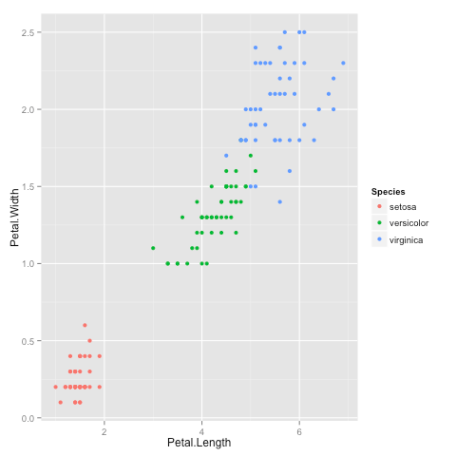
library(datasets)head(iris)  Sepal.Length Sepal.Width Petal.Length Petal.Width Species1          5.1         3.5          1.4         0.2  setosa2          4.9         3.0          1.4         0.2  setosa3          4.7         3.2          1.3         0.2  setosa4          4.6         3.1          1.5         0.2  setosa5          5.0         3.6          1.4         0.2  setosa6          5.4         3.9          1.7         0.4  setosaAfter a little bit of exploration, I found that Petal.Length and Petal.Width were similar among the same species but varied considerably between different species, as demonstrated below:
library(ggplot2)ggplot(iris, aes(Petal.Length, Petal.Width, color = Species)) + geom_point()Here is the plot:

ClusteringOkay, now that we have seen the data, let us try to cluster it. Since the initial cluster assignments are random, let us set the seed to ensure reproducibility.
set.seed(20)irisCluster <- kmeans(iris[, 3:4], 3, nstart = 20)irisClusterK-means clustering with 3 clusters of sizes 46, 54, 50Cluster means:  Petal.Length Petal.Width1     5.626087    2.0478262     4.292593    1.3592593     1.462000    0.246000Clustering vector:  [1] 3 3 3 3 3 3 3 3 3 3 3 3 3 3 3 3 3 3 3 3 3 3 3 3 3 3 3 3 3 3 3 3 3 3 [35] 3 3 3 3 3 3 3 3 3 3 3 3 3 3 3 3 2 2 2 2 2 2 2 2 2 2 2 2 2 2 2 2 2 2 [69] 2 2 2 2 2 2 2 2 2 1 2 2 2 2 2 1 2 2 2 2 2 2 2 2 2 2 2 2 2 2 2 2 1 1[103] 1 1 1 1 2 1 1 1 1 1 1 1 1 1 1 1 1 2 1 1 1 2 1 1 2 2 1 1 1 1 1 1 1 1[137] 1 1 2 1 1 1 1 1 1 1 1 1 1 1Within cluster sum of squares by cluster:[1] 15.16348 14.22741  2.02200 (between_SS / total_SS =  94.3 %)Available components:[1] "cluster"      "centers"      "totss"        "withinss"    [5] "tot.withinss" "betweenss"    "size"         "iter"        [9] "ifault"Since we know that there are 3 species involved, we ask the algorithm to group the data into 3 clusters, and since the starting assignments are random, we specify nstart = 20. This means that R will try 20 different random starting assignments and then select the one with the lowest within cluster variation.
We can see the cluster centroids, the clusters that each data point was assigned to, and the within cluster variation.
Let us compare the clusters with the species.
table(irisCluster$cluster, iris$Species)    setosa versicolor virginica  1      0          2        44  2      0         48         6  3     50          0         0As we can see, the data belonging to the setosa species got grouped into cluster 3, versicolor into cluster 2, and virginica into cluster 1. The algorithm wrongly classified two data points belonging to versicolor and six data points belonging to virginica.
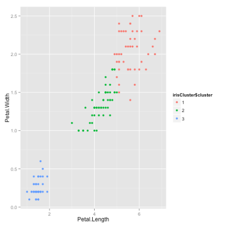
We can also plot the data to see the clusters:
irisCluster$cluster <- as.factor(irisCluster$cluster)ggplot(iris, aes(Petal.Length, Petal.Width, color = iris$cluster)) + geom_point()Here is the plot:

That brings us to the end of the article. I hope you enjoyed it! If you have any questions or feedback, feel free to leave a comment or reach out to me on Twitter.

扫码加我 拉你入群

请注明：姓名-公司-职位

以便审核进群资格，未注明则拒绝

分享0 收藏1 回帖

关键词：Analysis Cluster Analysi kmeans Analys google everyone 分析师 文章 博客