Want to know about Bayesian machine learning? Sure you do! Get a great introductory explanation here, as well as suggestions where to go for further study.
By Zygmunt Zając, FastML.
So you know the Bayes rule. How does it relate to machine learning? It can be quite difficult to grasp how the puzzle pieces fit together - we know it took us a while. This article is an introduction we wish we had back then.
While we have some grasp on the matter, we’re not experts, so the following might contain inaccuracies or even outright errors. Feel free to point them out, either in the comments or privately.
Bayesians and Frequentists
In essence, Bayesian means probabilistic. The specific term exists because there are two approaches to probability. Bayesians think of it as a measure of belief, so that probability is subjective and refers to the future.
Frequentists have a different view: they use probability to refer to past events - in this way it’s objective and doesn’t depend on one’s beliefs. The name comes from the method - for example: we tossed a coin 100 times, it came up heads 53 times, so the frequency/probability of heads is 0.53.
For a thorough investigation of this topic and more, refer to Jake VanderPlas’ Frequentism and Bayesianism series of articles.
Priors, updates, and posteriors
As Bayesians, we start with a belief, called a prior. Then we obtain some data and use it to update our belief. The outcome is called a posterior. Should we obtain even more data, the old posterior becomes a new prior and the cycle repeats.
This process employs the Bayes rule:
P( A | B ) = P( B | A ) * P( A ) / P( B )
P( A | B ), read as “probability of A given B”, indicates a conditional probability: how likely is A if B happens.
Inferring model parameters from data
In Bayesian machine learning we use the Bayes rule to infer model parameters (theta) from data (D):
P( theta | D ) = P( D | theta ) * P( theta ) / P( data )
All components of this are probability distributions.
P( data ) is something we generally cannot compute, but since it’s just a normalizing constant, it doesn’t matter that much. When comparing models, we’re mainly interested in expressions containing theta, because P( data ) stays the same for each model.
P( theta ) is a prior, or our belief of what the model parameters might be. Most often our opinion in this matter is rather vague and if we have enough data, we simply don’t care. Inference should converge to probable theta as long as it’s not zero in the prior. One specifies a prior in terms of a parametrized distribution - see Where priors come from.
P( D | theta ) is called likelihood of data given model parameters. The formula for likelihood is model-specific. People often use likelihood for evaluation of models: a model that gives higher likelihood to real data is better.
Finally, P( theta | D ), a posterior, is what we’re after. It’s a probability distribution over model parameters obtained from prior beliefs and data.
When one uses likelihood to get point estimates of model parameters, it’s called maximum-likelihood estimation, or MLE. If one also takes the prior into account, then it’s maximum a posteriori estimation (MAP). MLE and MAP are the same if the prior is uniform.
Note that choosing a model can be seen as separate from choosing model (hyper)parameters. In practice, though, they are usually performed together, by validation.
Model vs inference
Inference refers to how you learn parameters of your model. A model is separate from how you train it, especially in the Bayesian world.
Consider deep learning: you can train a network using Adam, RMSProp or a number of other optimizers. However, they tend to be rather similar to each other, all being variants of Stochastic Gradient Descent. In contrast, Bayesian methods of inference differ from each other more profoundly.
The two most important methods are Monte Carlo sampling and variational inference. Sampling is a gold standard, but slow. The excerpt from The Master Algorithm has more on MCMC.
Variational inference is a method designed explicitly to trade some accuracy for speed. It’s drawback is that it’s model-specific, but there’s light at the end of the tunnel - see the section on software below and Variational Inference: A Review for Statisticians.
Statistical modelling
In the spectrum of Bayesian methods, there are two main flavours. Let’s call the first statistical modelling and the second probabilistic machine learning. The latter contains the so-called nonparametric approaches.
Modelling happens when data is scarce and precious and hard to obtain, for example in social sciences and other settings where it is difficult to conduct a large-scale controlled experiment. Imagine a statistician meticulously constructing and tweaking a model using what little data he has. In this setting you spare no effort to make the best use of available input.
Also, with small data it is important to quantify uncertainty and that’s precisely what Bayesian approach is good at.
Bayesian methods - specifically MCMC - are usually computationally costly. This again goes hand-in-hand with small data.
To get a taste, consider examples for the Data Analysis Using Regression Analysis and Multilevel/Hierarchical Models book. That’s a whole book on linear models. They start with a bang: a linear model with no predictors, then go through a number of linear models with one predictor, two predictors, six predictors, up to eleven.
This labor-intensive mode goes against a current trend in machine learning to use data for a computer to learn automatically from it.
Probabilistic machine learning
Let’s try replacing “Bayesian” with “probabilistic”. From this perspective, it doesn’t differ as much from other methods. As far as classification goes, most classifiers are able to output probabilistic predictions. Even SVMs, which are sort of an antithesis of Bayesian.
By the way, these probabilities are only statements of belief from a classifier. Whether they correspond to real probabilities is another matter completely and it’s called calibration.
LDA, a generative model
Latent Dirichlet Allocation is a method that one throws data at and allows it to sort things out (as opposed to manual modelling). It’s similar to matrix factorization models, especially non-negative MF. You start with a matrix where rows are documents, columns are words and each element is a count of a given word in a given document. LDA “factorizes” this matrix of size n x d into two matrices, documents/topics (n x k) and topics/words (k x d).
The difference from factorization is that you can’t multiply those two matrices to get the original, but since the appropriate rows/columns sum to one, you can “generate” a document. To get the first word, one samples a topic, then a word from this topic (the second matrix). Repeat this for a number of words you want. Notice that this is a bag-of-words representation, not a proper sequence of words.
The above is an example of a generative model, meaning that one can sample, or generate examples, from it. Compare with classifiers, which usually model P( y | x ) to discriminate between classes based on x. A generative model is concerned with joint distribution of y and x, P( y, x ). It’s more difficult to estimate that distribution, but it allows sampling and of course one can get P( y | x ) from P( y, x ).
Bayesian nonparametrics
While there’s no exact definition, the name means that the number of parameters in a model can grow as more data become available. This is similar to Support Vector Machines, for example, where the algorithm chooses support vectors from the training points. Nonparametrics include Hierarchical Dirichlet Process version of LDA, where the number of topics chooses itself automatically, and Gaussian Processes.
Gaussian processes are somewhat similar to Support Vector Machines - both use kernels and have similar scalability (which has been vastly improved throughout the years by using approximations). A natural formulation for GP is regression, with classification as an afterthought. For SVM it’s the other way around.
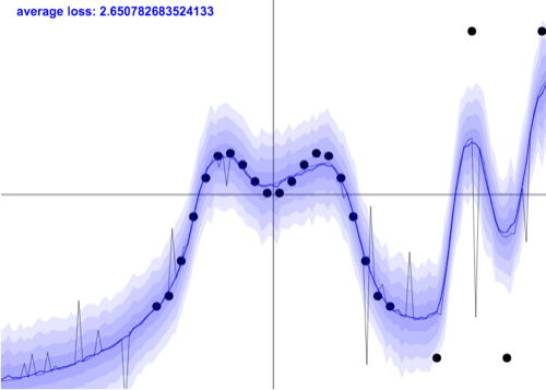
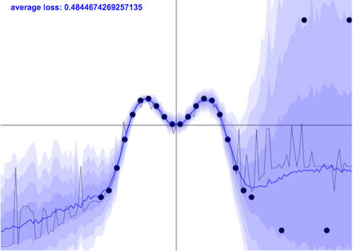
Another difference is that GP are probabilistic from the ground up (providing error bars), while SVM are not. You can observe this in regression. Most “normal” methods only provide point estimates. Bayesian counterparts, like Gaussian processes, also output uncertainty estimates.

Unfortunately, it’s not the end of the story. Even a sophisticated method like GP normally operates on an assumption of homoscedasticity, that is, uniform noise levels. In reality, noise might differ across input space (be heteroscedastic) - see the image below.


 395 个论坛币

 雷达卡
雷达卡


 京公网安备 11010802022788号


